Team II Gene Prediction Group: Difference between revisions
Siulung2005 (talk | contribs) |
|||
| (21 intermediate revisions by 4 users not shown) | |||
| Line 12: | Line 12: | ||
===Data=== | ===Data=== | ||
We are given 258 assembled genomes of Klebsiella spp. | We are given 258 assembled genomes of ''Klebsiella spp''. | ||
===Approach=== | ===Approach=== | ||
| Line 24: | Line 24: | ||
2. Statistical description of coding regions. | 2. Statistical description of coding regions. | ||
'''Hidden Markov Model (HMM)''' | |||
Hidden Markov Model (HMM) is a statistical Markov model in which the system being modeled is assumed to be a Markov process with unobserved (i.e. hidden) states. | Hidden Markov Model (HMM) is a statistical Markov model in which the system being modeled is assumed to be a Markov process with unobserved (i.e. hidden) states. | ||
[[File: Hmm.png|400px]] | |||
The room contains urns X1, X2, X3, … each of which contains a known mix of balls, each ball labeled y1, y2, y3, … . The genie chooses an urn in that room and randomly draws a ball from that urn. The Markov process itself cannot be observed, only the sequence of labeled balls, thus this arrangement is called a "hidden Markov process". This is illustrated by the lower part of the diagram shown in figure above, where one can see that balls y1, y2, y3, y4 can be drawn at each state. Even if the observer knows the composition of the urns and has just observed a sequence of three balls, e.g. y1, y2 and y3 on the conveyor belt, the observer still cannot be sure which urn (i.e., at which state) the genie has drawn the third ball from. However, the observer can work out other information, such as the likelihood that the third ball came from each of the urns. | |||
===Prodigal=== | ===Prodigal=== | ||
| Line 39: | Line 42: | ||
[[File: prodigal.jpg|500px]] | [[File: prodigal.jpg|500px]] | ||
'''Dynamic programming connection''' | |||
Red Arrows: Gene Connections | |||
Black Arrows: Intergenic Connections | |||
Blue Pieces: Potential Genes | |||
===GeneMarkS=== | ===GeneMarkS=== | ||
| Line 48: | Line 56: | ||
'''G'''ene '''L'''ocator and '''I'''nterpolated '''M'''arkov '''M'''odel'''er''' | '''G'''ene '''L'''ocator and '''I'''nterpolated '''M'''arkov '''M'''odel'''er''' | ||
Developed at ‘The Institute of Genomic Research (TIGR)’. | Developed at ‘The Institute of Genomic Research (TIGR)’. It's based on Interpolated (variable-order) Markov Model. | ||
UNIX program that uses the IMM algorithm to predict potential coding regions. | UNIX program that uses the IMM algorithm to predict potential coding regions. | ||
It's based on Interpolated (variable-order) Markov Model | It's based on Interpolated (variable-order) Markov Model | ||
| Line 54: | Line 62: | ||
1. Model Building | 1. Model Building | ||
2. Computation | 2. Computation | ||
It's easy to install, plenty of options, useful scripts included, relatively fast; | |||
Glimmer3 scores orfs in the reverse direction, i.e., 3’ to 5’; | |||
it has 2 step process; | |||
it builds a probability model of coding sequences, (different ways, one way is From long, non-overlapping orfs in the genome itself)
, then analyze sequence, make gene predictions
| |||
it gives you .predict .detail files, not GFF files. | |||
==Comparative== | ==Comparative== | ||
| Line 81: | Line 95: | ||
==RNA Prediction== | ==RNA Prediction== | ||
Non-coding RNA is the term used for RNA that gets transcribed from a DNA template but not translated into a protein, Three main classes | Non-coding RNA is the term used for RNA that gets transcribed from a DNA template but not translated into a protein, Three main classes of bacteria: tRNA/tmRNA, rRNA, and sRNA. Non-coding RNAs in bacterial genomes have been found to play a role in Protein synthesis/Translation (tRNA and rRNA), Gene regulation (sRNA) and both of them can be related to antibiotic resistance. | ||
===Rfam=== | ===Rfam=== | ||
Version: | Version: Rfam 13.0; Infernal 1.1.2<br> | ||
Input: | Rfam is an up-to-date ncRNA database that contains families of structural RNA sequences. In Rfam, covariance models (CMs) have been built for each family. To predict and annotate query sequences, infernal is used to build a CM of queries and compare to the CMs in Rfam database. | ||
<div style="border: 1pt dashed black; background : grey; padding: 1em 1em;"> | |||
Input: Rfam.clanin Rfam.cm INPUT.fasta<br> | |||
Output: OUTPUT.tblout and OUTPUT.cmscan | |||
</div> | |||
Performance by using reference genome:<br> | |||
<div style="border: 1pt dashed black; background : grey; padding: 1em 1em;"> | |||
Run-time: ~30mins for a 5.5Mb genome<br> | |||
ncRNA found: 286 | |||
</div> | |||
===Aragorn=== | ===Aragorn=== | ||
| Line 120: | Line 143: | ||
'''Figure 5: AUB=A+B-(A∩B)''' | '''Figure 5: AUB=A+B-(A∩B)''' | ||
== | ==Result== | ||
Next step was the validation; for which we used blast+ command line tool. We used the references that the genome assembly group used for Klebsiella species and extracted the gff files and then created a database using makeblastdb. Then we queried our predicted genes against this big database and picked up the top blast hits with this highest identity and highest length. Then we compared the number of predicted and number of blast hits. | |||
The following venn diagram explains the approach. The outer box is the number of predicted genes, the number of genes hit in blast and the difference or the shaded region could be the false positives or likely novel genes. This venn diagram can be translated to the plot on the right. we can confirm the percentage of hits for our tools lying between 80-95%. We used this to have a consistent metric for our validation from all the tools | |||
[[File: Venn.png|900px]] | |||
Then, we want to check the distribution of the gene prediction in the coding regions in both tools. | |||
[[File: GeneMarkS_hist.png|550px]] vs [[File: Prodigal_hist.png|550px]] | |||
The result of gene prediction for each individual sample in the both tools Prodigal and GeneMarkS and their consensus are compared the following. | |||
[[File: Intersecting_LinePlot.png|700px]] | |||
Prediction results for the noncoding regions is as following. | |||
'''tRNA''' | |||
All these three tools can tRNAs, This picture is using boxplot to compare the number of tRNAs predicted by there tools. <br>The x-axis shows tools, the y-axis shows the number of predicted tRNAs for every genome. <br>Comparing with Rfam and Aragorn, tRNAscan gives us the most hits.<br><br> | |||
[[File:TRNAs.png|600px]] | |||
'''tmRNA''' | |||
Both Aragorn and Rfam can predict tmRNA, in this picture both Rfam and Aragorn have only one line in its boxplot.<br> It tells that both of them predicts exactly one gene for every genome. Their results are very consistent.<br><br> | |||
[[File:TmRNAs.png|600px]] | |||
Final results after putting the prediction of the coding and noncoding regions together. | |||
[[File: AbInit_ncRna_Blast.png|700px]] | |||
==Final Pipeline== | |||
[[File: Final-pipeline.png]] | |||
'''Pipeline Options''' | |||
'''-f''' The fast version of the pipeline will be run | |||
GeneMark-S will not be run → GeneMark HMM will be run instead | |||
GeneMark-S: Creates a model for every genome → More accurate! | |||
GeneMark-HMM: Creates one model and uses it for all genomes | |||
Rfam will not be run (could affect sRNA predictions) | |||
'''-t''' The temporary files will be kept | |||
Results from all tools | |||
Results from all merging steps | |||
'''-v''' Verbose mode | |||
Latest revision as of 20:54, 6 April 2018
Introduction
Gene Prediction
In computational biology, gene prediction refers to the process of identifying the regions of genomic DNA that encode genes. This includes protein-coding genes as well as RNA genes, but may also include prediction of other functional elements such as regulatory regions. Gene prediction is one of the first and most important steps in understanding the genome of a species once it has been sequenced here.
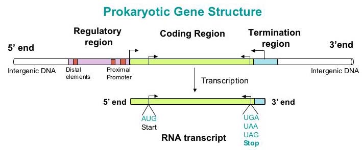
Before we move too far into gene prediction, we must understand the biological context. Genes are fragments of DNA that encodes a functional molecule, usually a protein. In order to go from a nucleotide sequence to a functional protein, the sequence must be transcribed and then translated. Genes always begin with a "start" codon (a specific sequence of three nucleotides), which serve to denote the beginning of a DNA sequence that encodes a protein. Prokaryotic genomes have a high gene density and do not contain introns in their protein coding regions, meaning that the prediction of prokaryotic genes tends to be relatively simpler.
Data
We are given 258 assembled genomes of Klebsiella spp.
Approach
Gene prediction by computational methods for finding the location of protein coding regions is one of the essential issues in bioinformatics. There are two basic problems in gene prediction: (1) prediction of protein coding regions and (2) prediction of the functional sites of genes. Two classes of methods are generally adopted: ab-initio prediction and comparative based searches that we explain them in the following here.
Ab-initio Prediction
Ab initio prediction is the challenging attempt to predict protein structures based only on sequence information and without using templates. it relies on two major features: 1. Gene signals (start and stop codon, intron splice signals, codon structure, etc.) 2. Statistical description of coding regions.
Hidden Markov Model (HMM)
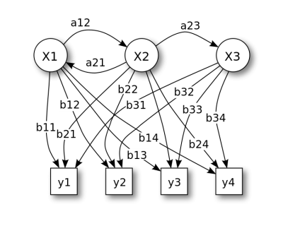
Hidden Markov Model (HMM) is a statistical Markov model in which the system being modeled is assumed to be a Markov process with unobserved (i.e. hidden) states.
The room contains urns X1, X2, X3, … each of which contains a known mix of balls, each ball labeled y1, y2, y3, … . The genie chooses an urn in that room and randomly draws a ball from that urn. The Markov process itself cannot be observed, only the sequence of labeled balls, thus this arrangement is called a "hidden Markov process". This is illustrated by the lower part of the diagram shown in figure above, where one can see that balls y1, y2, y3, y4 can be drawn at each state. Even if the observer knows the composition of the urns and has just observed a sequence of three balls, e.g. y1, y2 and y3 on the conveyor belt, the observer still cannot be sure which urn (i.e., at which state) the genie has drawn the third ball from. However, the observer can work out other information, such as the likelihood that the third ball came from each of the urns.
Prodigal
Prodigal is extremely fast and lightweight; also highly Specific - False positive rate < 5%; a distinct advantage of Prodigal over other gene-finders is that it performs well with high GC content genomes.
The results from Prodigal could be biased, because it was developed using results from GenBank annotation and using a small set of initial genomes; Recognition of short and atypical genes needs improvement.
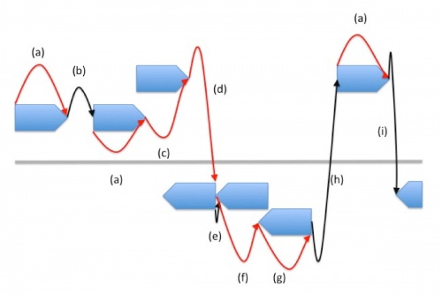
Dynamic programming connection Red Arrows: Gene Connections Black Arrows: Intergenic Connections Blue Pieces: Potential Genes
GeneMarkS
GeneMarkS is a new gene prediction method, utilizes a non-supervised training procedure and can be used for a newly sequenced prokaryotic genome with no prior knowledge of any protein or rRNA genes. The GeneMarkS implementation uses an improved version of the gene finding program GeneMark.hmm, heuristic Markov models of coding and non-coding regions and the Gibbs sampling multiple alignment program. GeneMarkS can be used (self-trained program). Longer than 50kb sequences to be provided. If shorter sequences, GeneMark heuristic program can be used with loss of some accuracy. Also it can generate multiple output format, including off, fna, faa, etc. However in this case, GeneMarkS is very slow.
Glimmer
Gene Locator and Interpolated Markov Modeler Developed at ‘The Institute of Genomic Research (TIGR)’. It's based on Interpolated (variable-order) Markov Model. UNIX program that uses the IMM algorithm to predict potential coding regions. It's based on Interpolated (variable-order) Markov Model Two Steps: 1. Model Building 2. Computation
It's easy to install, plenty of options, useful scripts included, relatively fast; Glimmer3 scores orfs in the reverse direction, i.e., 3’ to 5’; it has 2 step process; it builds a probability model of coding sequences, (different ways, one way is From long, non-overlapping orfs in the genome itself) , then analyze sequence, make gene predictions it gives you .predict .detail files, not GFF files.
Comparative
Comparative, similarity based or Homology based gene prediction uses previously sequenced genes and their protein products as a template for recognition of unknown genes in a newly sequenced DNA fragments. So, in short we cab say: It is using "Known Genes" to predict "New Genes".
Recently, the number of sequenced genomes has increased drastically and 99% of genes have homologous partner, 80% have orthologous partner and 85% identity (protein coding DNA) versus 69% identity (intronic DNA). All these can be considered as the motivation of using this method of gene prediction.
Given a known gene and an unannotated genome sequence, find a set of substrings in the genomic sequence whose concatenation best matches the known gene
Sequence alignment is a way of arranging the sequences to identify regions of similarity that may be results of functional, structural or evolutionary relationships between the genomes. Two methods based on similarity research are: Local alignment and Global alignment.
Local alignment tries to match your query with a substring of your reference. Smith–Waterman algorithm is based on local alignment. While, global alignment forces the alignment to span the entire length of all query sequences. It is most useful when the sequences are similar and roughly "equal size". Otherwise, it may end up with a lot of gaps. Needleman–Wunsch algorithmBased on Dynamic programing uses global alignment.
On the left, we have Local Alignment with 2 mismatch and 0 gaps. On the right, we have Global Alignment with 1 mismatch and 2 gaps of length 4 and 2
There are some tools for gene prediction based on comparative method such as "SGP2", "TwinScan" and "GenomeScan". But, they are developed just for some limited number of species. For example, Twinscan is currently available for Mammals, Caenorhabditis (worm), Dicot plants, and Cryptococci. Therefore, we can not use them for our dataset.
Blast
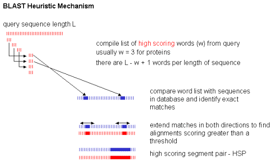
BLAST here for Basic Local Alignment Search Tool is an algorithm for comparing primary biological sequence information, such as the amino-acid sequences of proteins or the nucleotides of DNA sequences. A BLAST search enables a researcher to compare a query sequence with a library or database of sequences, and identify library sequences that resemble the query sequence above a certain threshold.
RNA Prediction
Non-coding RNA is the term used for RNA that gets transcribed from a DNA template but not translated into a protein, Three main classes of bacteria: tRNA/tmRNA, rRNA, and sRNA. Non-coding RNAs in bacterial genomes have been found to play a role in Protein synthesis/Translation (tRNA and rRNA), Gene regulation (sRNA) and both of them can be related to antibiotic resistance.
Rfam
Version: Rfam 13.0; Infernal 1.1.2
Rfam is an up-to-date ncRNA database that contains families of structural RNA sequences. In Rfam, covariance models (CMs) have been built for each family. To predict and annotate query sequences, infernal is used to build a CM of queries and compare to the CMs in Rfam database.
Input: Rfam.clanin Rfam.cm INPUT.fasta
Output: OUTPUT.tblout and OUTPUT.cmscan
Performance by using reference genome:
Run-time: ~30mins for a 5.5Mb genome
ncRNA found: 286
Aragorn
Version: aragorn1.2.38
Aragorn identifies tRNA and tmRNA genes. The program employs heuristic algorithms to predict tRNA secondary structure, based on homology with recognized tRNA consensus sequences and ability to form a base-paired cloverleaf.
Output: either FASTA or ARAGORN specific format
Performance by using reference genome:
Sensitivity: 98.4
Precision: 70.5
tRNAscan-SE 2.0
Version: tRNAscan-SE-2.0 and infernal-1.1.2
tRNAscan-SE was written in the PERL (version 5.0) script language.It searches for transfer RNAs in genomic sequence seqfile(s) using three separate methods to achieve a combination of speed, sensitivity, and selectivity not available with each program individually.
output: standard tabular, ACeDB-compatible or an extended format
Performance by using reference genome:
Sensitivity: 98.4
Precision: 68.1
Merge
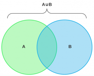
We use bedtools intersect to merge the two corresponding files from Prodigal and GeneMark. The entries from GeneMark predicted file, which do not overlap with any of the entry in the Prodigal predicted file, are concatenated to the latter file. We say that two entries do not overlap if they do not satisfy the 80% overlap criteria.
Figure 5: AUB=A+B-(A∩B)
Result
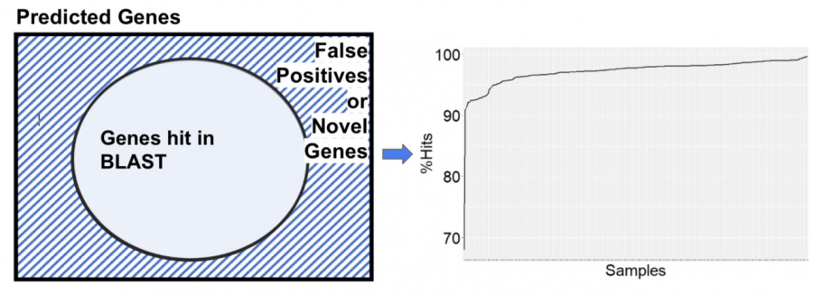
Next step was the validation; for which we used blast+ command line tool. We used the references that the genome assembly group used for Klebsiella species and extracted the gff files and then created a database using makeblastdb. Then we queried our predicted genes against this big database and picked up the top blast hits with this highest identity and highest length. Then we compared the number of predicted and number of blast hits.
The following venn diagram explains the approach. The outer box is the number of predicted genes, the number of genes hit in blast and the difference or the shaded region could be the false positives or likely novel genes. This venn diagram can be translated to the plot on the right. we can confirm the percentage of hits for our tools lying between 80-95%. We used this to have a consistent metric for our validation from all the tools
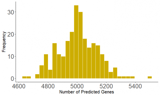
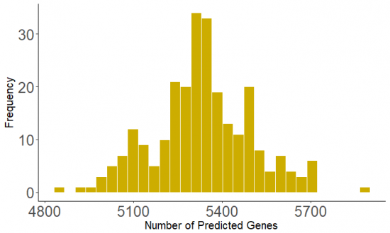
Then, we want to check the distribution of the gene prediction in the coding regions in both tools.
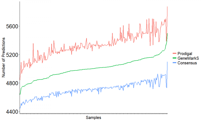
The result of gene prediction for each individual sample in the both tools Prodigal and GeneMarkS and their consensus are compared the following.
Prediction results for the noncoding regions is as following.
tRNA
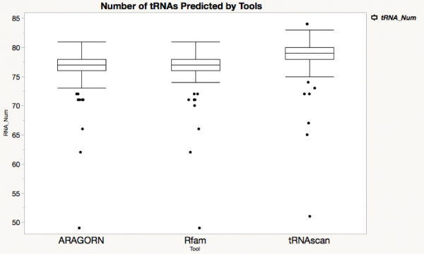
All these three tools can tRNAs, This picture is using boxplot to compare the number of tRNAs predicted by there tools.
The x-axis shows tools, the y-axis shows the number of predicted tRNAs for every genome.
Comparing with Rfam and Aragorn, tRNAscan gives us the most hits.
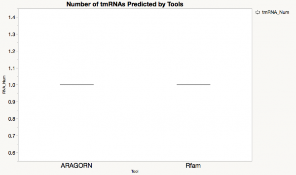
tmRNA
Both Aragorn and Rfam can predict tmRNA, in this picture both Rfam and Aragorn have only one line in its boxplot.
It tells that both of them predicts exactly one gene for every genome. Their results are very consistent.
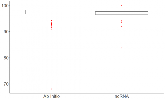
Final results after putting the prediction of the coding and noncoding regions together.
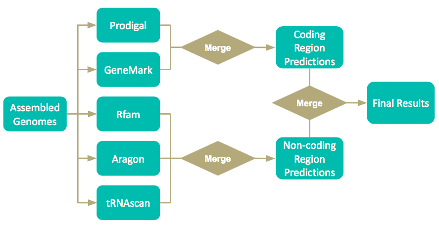
Final Pipeline
Pipeline Options
-f The fast version of the pipeline will be run GeneMark-S will not be run → GeneMark HMM will be run instead GeneMark-S: Creates a model for every genome → More accurate! GeneMark-HMM: Creates one model and uses it for all genomes Rfam will not be run (could affect sRNA predictions)
-t The temporary files will be kept
Results from all tools
Results from all merging steps
-v Verbose mode
