Team I Gene Prediction Group: Difference between revisions
| (16 intermediate revisions by 2 users not shown) | |||
| Line 5: | Line 5: | ||
===Data=== | ===Data=== | ||
We were given de Novo assemblies of 258 isolates of ''Klebsiella spp.''. | We were given "de Novo" assemblies of 258 isolates of ''Klebsiella spp.''. | ||
===Background=== | ===Background=== | ||
| Line 16: | Line 16: | ||
[[File:Team1_GP_ProkaryoticGene.jpg]] | [[File:Team1_GP_ProkaryoticGene.jpg]] | ||
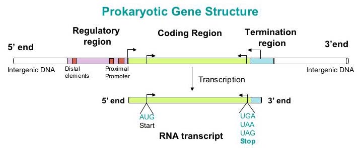
General structure of a prokaryotic gene. The start codons signify an ORF and are a strong signal for a potential coding region in prokaryotes. | |||
== '''Methods''' == | == '''Methods''' == | ||
| Line 36: | Line 39: | ||
<pre>makeblastdb -in reference.fasta -dbtype nucl -out db_name | <pre>makeblastdb -in reference.fasta -dbtype nucl -out db_name | ||
blastn -db db_name -query assembly_result.fasta -outfmt 6 -out blast_result.gff</pre> | blastn -db db_name -query assembly_result.fasta -outfmt 6 -out blast_result.gff</pre> | ||
''Reason why it didn’t work with assembly:'' | |||
BLAST searches if a potential gene has a match in database, it doesn’t work well with whole genome as input and whole genome as reference. A way to correct this is to break the assembly down by ORFfinder, but with ORFfinder finding all possible ORFs and returning too much ORFs that’s not actually potential genes, it’s not preferable in this case. | |||
The reference-based gene-finding actually was never supposed to work on whole genome assembly. It’s referred to the method of BLASTing a list of ORFs, without knowing if it’s a gene, against database to see if it’s actually a gene. In NCBI prokaryotes annotation pipeline, the raw assembly genome was first broke into ORFs by OFRfinder, then BLAST against protein database by BLASTp and later back to nucleotide database by tBLASTn, simply because the ORFs found were so rarely actual genes as they don’t have any gene features except for in-frame start and stop codon. Even so, the method cannot stand alone, and is mainly used as a correction or a helpful hand for GeneMarkS. | |||
=== Ab-initio Methods === | === Ab-initio Methods === | ||
Ab-initio tools always predict genes based on the gene content and signal detection(e.g. start/stop codon; Ribosome Biding Site, RBS etc.). In another words, they predict genes by analyzing statistical features of genes first, then separate the coding sequences and non-coding sequences apart. | Ab-initio tools always predict genes based on the gene content and signal detection(e.g. start/stop codon; Ribosome Biding Site, RBS etc.). In another words, they predict genes by analyzing statistical features of genes first, then separate the coding sequences and non-coding sequences apart. | ||
There are so many different algorithms among different ab-initio tools. For example, Dynamic programming gene finding, Hidden Markov Model, Interpolated Markov Model, Linear Discriminant Analysis and so on. By comparing the sensitive, PPV and running time, we chose some tools below to generate our final results. | There are so many different algorithms among different ab-initio tools. For example, Dynamic programming gene finding, Hidden Markov Model, Interpolated Markov Model, Linear Discriminant Analysis and so on. By comparing the sensitive, PPV and running time, we chose some tools below to generate our final results. | ||
We chose the ab initio tools that we would use in our final pipeline from 10 sample assemblies that were given to us by the Team 1 Assembly group. They used a MASH tree to map the 10 assemblies to a reference, and we used those gene references to test the sensitivity and specificity. | |||
We calculated these values by calculating with BLAST the genes with over 99% identical matches and over 100 bp alignment length. With these blast results, we calculated the sensitivity and positive predictive value. Because we cannot calculate the number of true negatives in our predicted genes, the positive predictive value is instead a measure of how confident we are in the genes we predicted. | |||
<li> Sensitivity: TP / (TP + FN) </li> | |||
<li> Positive Predictive value: PPV = TP/ (TP + FP) </li> | |||
[[File:TableSensitivity.png|500px]] | |||
Because the tools all performed well in sensitivity and PPV, we chose to go forward with Prodigal, GeneMark HMM, and Glimmer for our final pipeline. | |||
'''Prodigal''' | '''Prodigal''' | ||
| Line 131: | Line 153: | ||
'''RNAMMER''' | '''RNAMMER''' | ||
RNAmmer is a widely used ribosomal RNA prediction tool, it accepts both Prokaryotic and Eukaryotic inputs and returns result in gff, fasta and html formats based on need. | RNAmmer is a widely used ribosomal RNA prediction tool, it accepts both Prokaryotic and Eukaryotic inputs and returns result in gff, fasta and html formats based on need. By using hidden markov models trained on two databases(5S rRNA database and the european rRNA database project (ERRD)), RNAmmer can accurately locate rRNAs in genomes. | ||
“rnammer” is a wrapper used to initialize search, the “core-rnammer” is the core Perl program for this tool. | |||
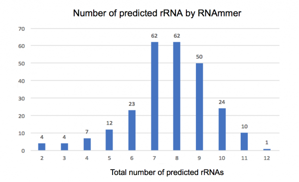
On average, we get 7 matches from RNAmmer in each genome, which is lower than what NCBI suggested (20~25). The reason for that is we used scaffolded genomes, each genome was broken into several parts, so that RNAs in the connecting part could not be identified. | |||
Command: | Command: | ||
<pre> rnammer -S bac -m lsu,ssu,tsu -multi -gff output_file.gff -f output_file.fasta < input.fasta </pre> | <pre> rnammer -S bac -m lsu,ssu,tsu -multi -gff output_file.gff -f output_file.fasta < input.fasta </pre> | ||
-S: kingdom, specify if input file is prokaryotes or eukaryotes | |||
-m: molecule type (lsu: 23/28s rRNA; ssu: 16/18s rRNA; tsu:5/8s rRNA) | |||
-multi: run both strands in parallel | |||
-gff: gff format output | |||
-f: fasta format output | |||
(optional) -h: html format output | |||
== ''' Validation ''' == | == ''' Validation ''' == | ||
| Line 161: | Line 199: | ||
We reported all of the tRNA and rRNA results because the genes are highly conserved and so we can be confident that those sequences are present if they are predicted, though their function may not be relevant. Only BLAST could be used to verify if our predicted istR genes have been seen before. This approach could give us more confidence in true positives but will call a never before seen gene as not real. Therefore the istR results were not run through BLAST. | We reported all of the tRNA and rRNA results because the genes are highly conserved and so we can be confident that those sequences are present if they are predicted, though their function may not be relevant. Only BLAST could be used to verify if our predicted istR genes have been seen before. This approach could give us more confidence in true positives but will call a never before seen gene as not real. Therefore the istR results were not run through BLAST. | ||
[[File:Table_unionGP1.png|600px]] | |||
== ''' Results ''' == | == ''' Results ''' == | ||
| Line 169: | Line 209: | ||
'''Results''' | '''Results''' | ||
'''Gene Prediction''' | '''Gene Prediction''' | ||
| Line 183: | Line 217: | ||
[[File:Prodigal_results.png|600px]] | [[File:Prodigal_results.png|600px]] | ||
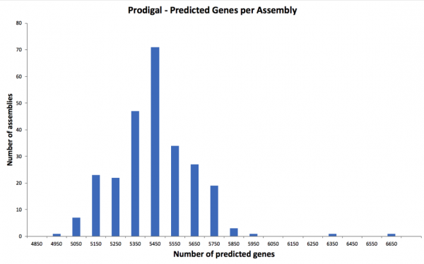
Distribution of gene count predicted for all assemblies using Prodigal. The average number of predicted genes per assembly was 5374. | |||
GeneMark HMM | GeneMark HMM | ||
[[File:Genemark_HMM.png|600px]] | [[File:Genemark_HMM.png|600px]] | ||
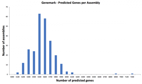
Distribution of gene count predicted for all assemblies using Genemark HMM. The average number of predicted genes per assembly was 5515. | |||
'''Non-coding RNA''' | '''Non-coding RNA''' | ||
| Line 193: | Line 233: | ||
[[File:RNAmmer results.png|600px]] | [[File:RNAmmer results.png|600px]] | ||
Distribution of rRNA count predicted for all assemblies using RNAmmer. The average number of predicted genes per assembly was 8. | |||
Infernal | Infernal | ||
| Line 205: | Line 249: | ||
[[File:Aragorn results.png|600px]] | [[File:Aragorn results.png|600px]] | ||
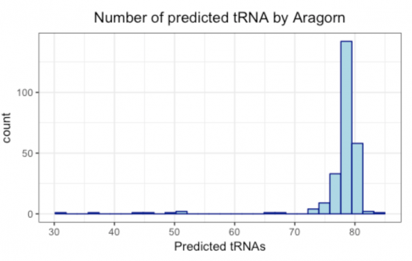
Distribution of tRNA count predicted for all assemblies using Aragorn. . The average of tRNA predicted was 77 with a standard deviation of 6. The average running time was 2-4 seconds per genome. | |||
== ''' Conclusion '''== | |||
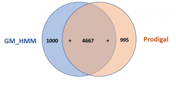
In our pipeline, we report the results in GFF3 format, fasta, and fasta amino acid formats for protein coding genes. Here is a figure representing the average for each of our genomes: | |||
[[File:VenDiagram.png|600px]] | |||
Because we chose to not get rid of the genes from either of the tools, on average we report 6662 genes for each genome. These will be passed to the functional annotation group so they can predict the functions and find antibiotic resistance features. | |||
== '''References''' == | == '''References''' == | ||
Latest revision as of 20:57, 27 March 2018
Team members: Genevieve Brandt, Victoria Caban, Yuntian He, Junyu Li, Yiqiuyi Liu, Yihao Ou, Wenyi Qiu, Casey Smith, Mohit Thakur, Stephen Wist, Qinyu Yue
Introduction
Data
We were given "de Novo" assemblies of 258 isolates of Klebsiella spp..
Background
Our overarching goal is to understand what causes heteroresistance in Klebsiella spp. At this step, our objective was, given assembled genomes, to predict genes for Klebsiella that could later be annotated to understand functionality.
Gene Prediction
Gene prediction is the process of identifying the specific regions of genomic DNA that encode for genes. After sequencing and assembly, gene prediction is one of the first steps in understanding the genome of a species. In the past, confirming that the gene prediction is accurate demanded in vivo experimentation through gene knockout and other assays. Today, bioinformatics research has made it possible to predict the function of a gene based on its sequence alone. There are two general methods to do this: homology-based tools and ab-initio tools.
There is a big difference between prokaryotic and eukaryotic gene prediction. For eukaryotes, genes may be separated by introns, which makes it challenging to find the whole genomic sequence. Promoter sequences are more complex and less well understood in eukaryotes as well. In prokaryotes, the promoter regions are well understood, which is useful when using ab initio tools, since these tools search for signs of specific signs of protein coding genes. In prokaryotic genomes there are also contiguous open reading frames (ORFs) - when paired with the high amount of stop codons in prokaryotes this can indicate, with high probability, a gene being present. Our challenge when looking at ORFs is that every gene is a ORF, but not every ORF is a gene.
General structure of a prokaryotic gene. The start codons signify an ORF and are a strong signal for a potential coding region in prokaryotes.
Methods
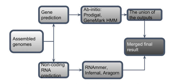
Pipeline (general workflow)
Homology-Based Methods
BLAST
One sequence by itself is not informative; it must be analyzed by comparative methods against existing sequence databases to develop hypothesis concerning relatives and function. BLAST(Basic Local Alignment Search Tool) is a widely used tool for similarity search, which adopts a Heuristic approach based on the Smith Waterman algorithm. BLAST provides not only the results of best local alignment, but various statistical significance as well.This algorithm compares a query sequence against reference sequence or specific database, such as nucleotide database. Because there are 258 assemblies that we are intending to BLAST, we chose to use local BLAST. The reference sequences we picked are the sequences which were used for gene assembly, the query sequences are the assembly results from Spades.
To run BLAST, we first need to create a database using the reference genome, then blast the query sequence against the database.
Commands:
makeblastdb -in reference.fasta -dbtype nucl -out db_name
blastn -db db_name -query assembly_result.fasta -outfmt 6 -out blast_result.gff
Reason why it didn’t work with assembly:
BLAST searches if a potential gene has a match in database, it doesn’t work well with whole genome as input and whole genome as reference. A way to correct this is to break the assembly down by ORFfinder, but with ORFfinder finding all possible ORFs and returning too much ORFs that’s not actually potential genes, it’s not preferable in this case.
The reference-based gene-finding actually was never supposed to work on whole genome assembly. It’s referred to the method of BLASTing a list of ORFs, without knowing if it’s a gene, against database to see if it’s actually a gene. In NCBI prokaryotes annotation pipeline, the raw assembly genome was first broke into ORFs by OFRfinder, then BLAST against protein database by BLASTp and later back to nucleotide database by tBLASTn, simply because the ORFs found were so rarely actual genes as they don’t have any gene features except for in-frame start and stop codon. Even so, the method cannot stand alone, and is mainly used as a correction or a helpful hand for GeneMarkS.
Ab-initio Methods
Ab-initio tools always predict genes based on the gene content and signal detection(e.g. start/stop codon; Ribosome Biding Site, RBS etc.). In another words, they predict genes by analyzing statistical features of genes first, then separate the coding sequences and non-coding sequences apart.
There are so many different algorithms among different ab-initio tools. For example, Dynamic programming gene finding, Hidden Markov Model, Interpolated Markov Model, Linear Discriminant Analysis and so on. By comparing the sensitive, PPV and running time, we chose some tools below to generate our final results.
We chose the ab initio tools that we would use in our final pipeline from 10 sample assemblies that were given to us by the Team 1 Assembly group. They used a MASH tree to map the 10 assemblies to a reference, and we used those gene references to test the sensitivity and specificity.
We calculated these values by calculating with BLAST the genes with over 99% identical matches and over 100 bp alignment length. With these blast results, we calculated the sensitivity and positive predictive value. Because we cannot calculate the number of true negatives in our predicted genes, the positive predictive value is instead a measure of how confident we are in the genes we predicted.
 Because the tools all performed well in sensitivity and PPV, we chose to go forward with Prodigal, GeneMark HMM, and Glimmer for our final pipeline.
Prodigal
Pros:
Cons:
Parameters used:
Input: assembly file (.fna) Output: gene coordinates (.gff), nucleotide sequences (.fna), protein sequences (.fna) Command:
prodigal -i input.fna -o output.gff -f gff -d nucleotide_seq.fna -a protein_seq.fna
Reference: Hyatt, Doug, et al. "Prodigal: prokaryotic gene recognition and translation initiation site identification." BMC bioinformatics 11.1 (2010): 119.
Genemark.hmm
Before running GeneMark.hmm, it is necessary to got a mode file first. One way is to download the models from GeneMark website(http://opal.biology.gatech.edu/GeneMark/). Or you can generated them by GeneMarkS or GeneMark.
Pros:
Input: assembly file (.fna) Output: gene coordinates (.gff), nucleotide sequences (.fna), protein sequences (.fna) Command:
gmhmmp -o <output.gff> -f G -m <model with its path> <input_file>
GLIMMER
Run_glimmer.sh includes:
- Add GLIMMER executables to PATH
- Create output and log directories GFF/ and logs/
- GLIMMER calling, done through a pipeline script GLIMMER3 provides g3-from-scratch.csh
- Convert GLIMMER outputs to GFFs
Parameters used: (default in g3-from-scratch.csh)
Input: directory of assembly FASTA file(s) Output: Gene table (.predict and .detail) and byproducts (.icm, .train, .longorfs) Command:
bash run_glimmer.sh [directory]
ncRNA Methods
Infernal
There exists large varieties of ncRNA beyond tRNA and rRNA that are important for biological function. Infernal is a de novo ncRNA prediction tool that can predict diverse families of ncRNA. Infernal compares nucleotide sequences against profiles, structually annotated multiple sequence alignments of RNA, to predict RNA sequences. Its compares both primary and secondary structure to increase its accuracy. These profiles use position specific scoring to account the importatnce of each insertions, deletions, and substitutions. Structural annotations can identify key residues which are dependent on each other. These profiles are implemented by Infernal as covariance models (CM), a specialized version of hidden markov models [1].
RFam is a database of RNA CMs information about RNA families [2]. The istR RNA CM was chosen based on its potential role in heteroresistance. The TisB-istR toxin-antitoxin system is induced by DNA damage and causes the cell to arrest growth rather than die [3]. This could be a cause of the ability of our heteroresistant and non-heteroresistant Klebsiella pneumoniae spp. To persist in environments it shouldn’t.
Infernal is a suite of many executables to create, manipulate, and analyze using covariance models. For our purposes we only needed to use the `cmscan` program. This command searches query sequences against a covariance model database.
Command:
cmscan --tblout <path to write tblout file> <cm file> <input fasta> > <path to write cmscan output>
Aragorn
A homology non coding RNA prediction tool, his program quickly identifies tRNA and tmRNA genes. It uses heuristic algorithms to predict tRNA secondary structure, based on homology with recognized tRNA consensus sequences. This program outputs reports ofthe proposed tRNA secondary structure and, for tmRNA genes, the secondary structure of the tRNA domain, the tmRNA gene sequence, the tag peptide and a list of organisms with matching tmRNA peptide tags.
Command:
./aragorn -t <input file>
RNAMMER
RNAmmer is a widely used ribosomal RNA prediction tool, it accepts both Prokaryotic and Eukaryotic inputs and returns result in gff, fasta and html formats based on need. By using hidden markov models trained on two databases(5S rRNA database and the european rRNA database project (ERRD)), RNAmmer can accurately locate rRNAs in genomes.
“rnammer” is a wrapper used to initialize search, the “core-rnammer” is the core Perl program for this tool.
On average, we get 7 matches from RNAmmer in each genome, which is lower than what NCBI suggested (20~25). The reason for that is we used scaffolded genomes, each genome was broken into several parts, so that RNAs in the connecting part could not be identified.
Command:
rnammer -S bac -m lsu,ssu,tsu -multi -gff output_file.gff -f output_file.fasta < input.fasta
-S: kingdom, specify if input file is prokaryotes or eukaryotes
-m: molecule type (lsu: 23/28s rRNA; ssu: 16/18s rRNA; tsu:5/8s rRNA)
-multi: run both strands in parallel
-gff: gff format output
-f: fasta format output
(optional) -h: html format output
Validation
Validation for Protein Coding Gene
After finding that all four tools we tested had high sensitivity and PPV, we decided to use a validation method in our final pipeline to utilize multiple tools. We wanted to choose a method that would predict genes of high confidence but also possibly with novel functions. So, we did not want to eliminate genes that were not in references. Our first method that we pursued was to use Glimmer, GeneMarkHMM, and Prodigal results to find genes that were predicted by more than one tool. However, we had problems with this method because the Glimmer results were not able to be merged with the other results. So, we next found the intersect between Gene Mark HMM and Prodigal. We used our 10 test assemblies with references to test this validation method.
From these results, we can see that through only choosing the intersect we were using a large portion of the true positives. In order to preserve the true positives and genes with possible novel functions, we instead wrote an algorithm to get the merged results of GeneMark HMM and Prodigal. We used bedtools intersect and found the intersect of the two files, and the unique genes from each output. We combined the intersect and unique genes into one output for our final results.
Commands used:
bedtools intersect -f 0.99 -r -wa -v -a prodigal_gff -b hmm_gff > "$3_complement.gff"
This command keeps any genes that are less than 99% similar for each other, using the format from the original gff file. We did this for both prodigal and hmm.
bedtools intersect -f 0.99 -r -a prodigal_gff -b hmm_gff > "intersect.gff"
By concatenating the intersect with the unique genes we were then able to get the union.
Validation of tRNA, rRNA, istR
We reported all of the tRNA and rRNA results because the genes are highly conserved and so we can be confident that those sequences are present if they are predicted, though their function may not be relevant. Only BLAST could be used to verify if our predicted istR genes have been seen before. This approach could give us more confidence in true positives but will call a never before seen gene as not real. Therefore the istR results were not run through BLAST.
Results
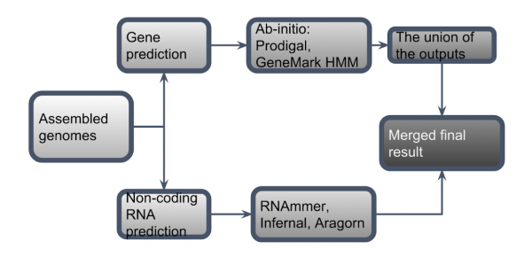
Final Pipeline
Results
Gene Prediction
Ab-initio
Prodigal
Distribution of gene count predicted for all assemblies using Prodigal. The average number of predicted genes per assembly was 5374.
GeneMark HMM
Distribution of gene count predicted for all assemblies using Genemark HMM. The average number of predicted genes per assembly was 5515.
Non-coding RNA
RNAmmer
Distribution of rRNA count predicted for all assemblies using RNAmmer. The average number of predicted genes per assembly was 8.
Infernal
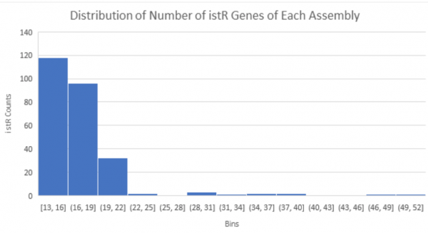
Histogram of istR counts found in each assembly. The majority of istR counts are between 13 and 19, with about 30 counts between 20 and 22, and a handful of high outliers. The outliers may be produced by assemblies with an abnormal amount of contigs and their accuracy is dubious. That most assemblies have multiple copies of istR may be indicative of its importance in Klebsiella spp.
Aragorn
Distribution of tRNA count predicted for all assemblies using Aragorn. . The average of tRNA predicted was 77 with a standard deviation of 6. The average running time was 2-4 seconds per genome.
Conclusion
In our pipeline, we report the results in GFF3 format, fasta, and fasta amino acid formats for protein coding genes. Here is a figure representing the average for each of our genomes:
Because we chose to not get rid of the genes from either of the tools, on average we report 6662 genes for each genome. These will be passed to the functional annotation group so they can predict the functions and find antibiotic resistance features.
References
https://ghr.nlm.nih.gov/primer/basics/gene
https://www.biostat.wisc.edu/bmi776/spring-15/lectures/IMMs.pdf
http://ece.drexel.edu/gailr/ECE-S690-503/markov_models.ppt.pdf
http://onlinelibrary.wiley.com/doi/10.1042/BC20070137/full#footer-citing
https://iweb.langara.bc.ca/biology/mario/Biol2315notes/biol2315chap11.h
http://opal.biology.gatech.edu/GeneMark/background.html
Lukashin, Alexander V., and Mark Borodovsky. "GeneMark. hmm: new solutions for gene finding." Nucleic acids research 26.4 (1998): 1107-1115
https://ccb.jhu.edu/software/glimmer/glim302notes.pdf
Nawrocki, E. P., and S. R. Eddy. “Infernal 1.1: 100-Fold Faster RNA Homology Searches.”Bioinformatics, vol. 29, no. 22, 2013, pp. 2933–2935., doi:10.1093/bioinformatics/btt509
Kalvari, I., Argasinska, J., Quinones-Olvera, N., Narwrocki, E. P., Rivas, E., Eddy, S. R., Bateman, A., Finn, R. D., and A. I. Petrov. “Rfam 13.0: shifting to a genome-centric resource for non-coding RNA families” Nucleic Acids Research, 2017, doi:12.1093/nar/gkx1038
Unoson, C., and E. G. H. Wagner. "A small SOS-induced toxin is targeted against the inner membrane in Escherichia coli". Molecular Microbiology, vol. 70, no .1, 2008, pp. 258–270. doi:10.1111/j.1365-2958.2008.06416.x
Lagesen K, et al. RNAmmer: consistent and rapid annotation of ribosomal RNA genes. Nucleic Acids Res. 2007;35:3100–3108. doi: 10.1093/nar/gkm160
