Team II Genome Assembly Group: Difference between revisions
No edit summary |
No edit summary |
||
| (157 intermediate revisions by 4 users not shown) | |||
| Line 2: | Line 2: | ||
=== Background === | === Background === | ||
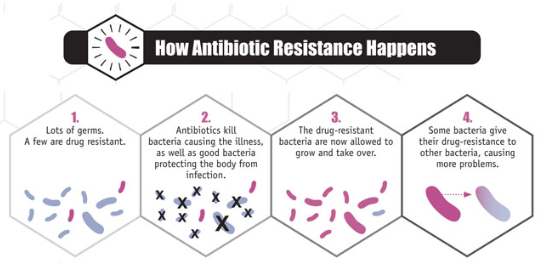
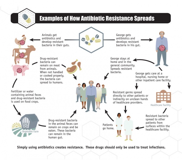
Antibiotic resistance has been called one of the world’s most pressing public health problems. | Antibiotic resistance has been called one of the world’s most pressing public health problems. It is the ability of bacteria to resist the effects of an antibiotic and occurs when bacteria change in a way that reduces the effectiveness of drugs, chemicals, or other agents designed to cure or prevent infections. The bacteria survive and continue to multiply, causing more harm (Figure 1.a.). Antibiotic resistance can cause illnesses that were once easily treatable with antibiotics to become dangerous infections, prolonging suffering for children and adults. Antibiotic-resistant bacteria can spread to family members, schoolmates, and co-workers, and may threaten your community (Figure 1.b). Antibiotic-resistant bacteria are often more difficult to kill and more expensive to treat and in some cases, can lead to serious disability or even death. | ||
[[File: | |||
'''Figure 1. How | [[File:1.png|50]] [[File:2.jpg|600px]] | ||
'''Figure 1:''' '''a.''' ''How antibiotic resistance happens, '' '''b.''' ''How antibiotic resistance spreads'' [https://www.cdc.gov/antibiotic-use/community/about/antibiotic-resistance-faqs.html here] | |||
=== Data === | === Data === | ||
Emory Antibiotic Resistance Center (ARC) in Emory University, School of medicine tries to better understand antibiotic resistance to combat this crisis and improve human health. Their goals include learning how antibiotic resistance develops, optimizing the way antibiotics are used to preserve their power, and discovering novel therapeutics and vaccines to directly combat antibiotic-resistant pathogens. Solving the crisis of antibiotic resistance requires a multi-faceted approach that crosses traditional boundaries [http://antibiotics.emory.edu/about/index.html here]. | |||
Dr. David S. Weiss' lab (ARC, Division of Infectious Diseases) provided us with a sample ID numbers and we downloaded 258 pair-end raw reads sequences of ''Klebsiella spp'',sequenced by illumina MiSeq. from NCBI SRA database. | |||
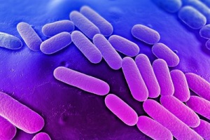
''Klebsiella'' is a genus of nonmotile, Gram-negative, oxidase-negative, rod-shaped bacteria (Figure 2) with a prominent polysaccharide-based capsule. ''Klebsiella'' species are found everywhere in nature. The members of the genus ''Klebsiella'' are a part of the human and animal's normal flora in the nose, mouth and intestines. The species of ''Klebsiella'' are all gram-negative and non-motile. They tend to be shorter and thicker when compared to others in the Enterobacteriaceae family. The cells are rods in shape and generally measures 0.3 to 1.5 µm wide by 0.5 to 5.0 µm long. They can be found singly, in pairs, in chains or linked end to end. ''Klebsiella'' can grow on ordinary lab medium and do not have special growth requirements, like the other members of Enterobacteriaceae. Some of ''Klebsiella'' types are: ''K.granulomatis'', ''K. oxytoca'', ''K. michiganensis'' and ''K. pneumoniae'' (type-species: ''K. p. subsp. ozaenae'', ''K. p. subsp. pneumoniae'', ''K. p. subsp. rhinoscleromatis'') [https://en.wikipedia.org/wiki/Klebsiella here]. Though, they have been extensively studied, for example, only four complete genomes of ''K. pneumoniae'' were available till 2011 [https://www.ncbi.nlm.nih.gov/pmc/articles/PMC3165360/ here]. To better understand the multidrug resistance factors in ''Klebsiella'', we need to determine genome DNA sequences of strains. | |||
[[File: 3.jpg | 300px]] | |||
'''Figure 2:''' ''Scanning electron microscope image of Klebsiella pneumoniae. From: Bioquell.com'' | |||
== Objectives == | == Objectives == | ||
The main objectives of the project is to distinguish between susceptible and heteroresistant strains/species, discover genomic determinants of antibiotic resistance and develop a predictive web server. Genome assembly group's objective, as the the first subgroup of the project, is to assemble the whole or contig genomes of DNA. | |||
== Pre-Assembly == | |||
Before doing any assembly, we would like to got some basic statistics about our dataset as: | |||
1. Per base sequence quality | |||
2. Per base N content | |||
3. Per base GC content | |||
4. Overrepresented sequences | |||
5. Sequence length distribution | |||
We use '''FastQC''' [https://www.bioinformatics.babraham.ac.uk/projects/fastqc/ here] for receiving these information and making some visualization. These kind of information will give us an overall view and help us to improve the quality of our sequences, if it is necessary, as raw inputs for the assemblers . For example, The presence of poor quality or technical sequences such as adapters in next-generation sequencing (NGS) data can easily affect the quality of assembly. We used '''Trim Galore''' [https://www.bioinformatics.babraham.ac.uk/projects/trim_galore/ here] and '''Sickle''' [https://github.com/najoshi/sickle here] to guarantee the best performance for each assembly method that we will use. | |||
''Trim Galore'' is a wrapper script to automate quality and adapter trimming as well as quality control. It specifically designed for Illumina data and has an Illumina adapter library. | |||
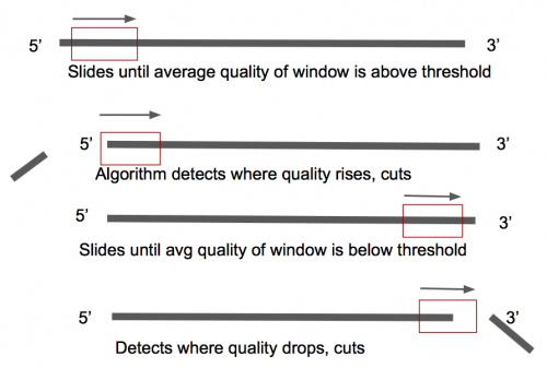
''Sickle'' is a tool that uses sliding windows along with quality and length thresholds to determine when quality is sufficiently low to trim the 3'-end of reads and also determines when the quality is sufficiently high enough to trim the 5'-end of reads (Figure 3). | |||
[[File: 5.png | 500px]] | |||
'''Figure 3:''' '' How Sickle is working'' | |||
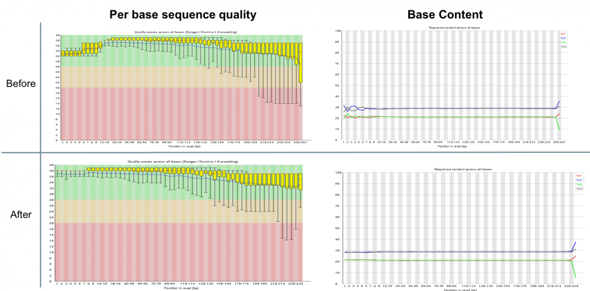
The results for before and after trimming of one of our samples shown in Figure 4. | |||
[[File: b_a.png | 1200px]] | |||
'''Figure 4:''' ''Per base sequence quality and Base content of one of the sample before and after trimming'' | |||
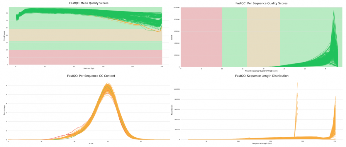
After trimming the adapter and the low quality reads, we can check the quality of all sequences at one with the '''MultiQC''' [http://multiqc.info here] tool. | |||
''MultiQC'' is a general use tool, perfect for summarising the output from numerous bioinformatics tools . | |||
[[File: MultiQC.png | 1180px]] | |||
'''Figure 5:''' ''Summary of trimmed reads from MultiQC'' | |||
== Assembly == | == Assembly == | ||
In bioinformatics, sequence assembly refers to aligning and merging fragments from a longer DNA sequence in order to reconstruct the original sequence. This is needed as DNA sequencing technology cannot read whole genomes in one go, but rather reads small pieces of between 20 and 30000 bases, depending on the technology used [https://en.wikipedia.org/wiki/Sequence_assembly here]. | |||
=== Reference Assembly === | |||
A type of genome assembly where the reads are mapped (or compared) to a known version of the organism’s genome. It saves time and is significantly more accurate and assemble the genome with less contigs. But, it has some disadvantage too. We would not discover new genes with this method of assembly, new (completely different) sequences may lost. It requires a reference that is very similar to the sequenced data. If multiple positions on the reference genome are equally likely for a read, then, reads are ignored, placed at multiple locations or placed at the first likely position. | |||
====Tool testing==== | |||
Most reference aligners use burrows-wheeler transform, which was initially developed as a compression algorithm. It is explained in detail [https://academic.oup.com/bioinformatics/article/25/14/1754/225615 here] . We decided to compare the burrows wheeler aligner with bowtie2, which aligns short reads using a seed-and-extend method. We aligned a small subset of our samples against a reference ''Klebsiella pneumoniae'' and ''Klebsiella oxytoca'' genome. | |||
{| class="wikitable" | |||
|- | |||
! '''Bowtie2''' | |||
! ''Klebsiella pneumoniae'' | |||
! ''Klebsiella oxytoca'' | |||
|- | |||
| Average time for one alignment | |||
| 17 minutes | |||
| 17 minutes | |||
|- | |||
| Genome fraction coverage | |||
| 97% | |||
| No conting larger than 7% | |||
|} | |||
{| class="wikitable" | |||
|- | |||
! '''bwa''' | |||
! ''Klebsiella pneumoniae'' | |||
! ''Klebsiella oxytoca'' | |||
|- | |||
| Average time for one alignment | |||
| 17 minutes | |||
| 26 minutes | |||
|- | |||
| Genome fraction coverage | |||
| 97% | |||
| No conting larger than 58% | |||
|} | |||
Based on the results above, we decided to proceed with bowtie2, as we found it to be less resource intensive. | |||
====Identifying suitable reference genomes==== | |||
As we don't know the species of the ''Klebsiella'', cannot simply choose a ''Klebsiella'' species to use as reference genome. Therefore, we need to find the reference genomes from the 250+ ''Klebsiella'' genomes which are closest related to our reads. For this aim, we used '''[https://bioconda.github.io/recipes/mashtree/README.html Mashtree]'''. It creates a tree based on Mash distance for our trimmed reads and 250+ ''Klebsiella'' genomes. Based on this Mashtree, we filtered to form a set of 51 representative reference. '''[http://bioinfo.ut.ee/strainseeker/ Strainseeker]''' is the tool that we used for strain identification. | |||
''StrainSeeker'' is a two step process: | |||
1) Building the database: We built a custom database with the filtered 51 references using the builder.pl script which takes input as references in fasta format and a newick reference guide tree. To generate the tree, we used [https://alurulab.cc.gatech.edu/phylo ALFRED-G] and converted it to a newick format for strainseeker input. | |||
2) Strain Identification: The trimmed fastq reads (either forwards or reverse or both) are input to the seeker.pl script which looks through the reference database and infers the identity. | |||
Results from StrainSeeker will tell us which ''Klebsiella'' strain is related to each single read. Based on these results we categorize all the reads into different bins based on the references and assemble that batch based on the assigned reference using [http://bowtie-bio.sourceforge.net/bowtie2/index.shtml Bowtie2]. | |||
=== De Novo Assembly === | === De Novo Assembly === | ||
De novo sequencing refers to sequencing a novel genome where there is no reference sequence available for alignment. Sequence reads are assembled as contigs, and the coverage quality of de novo sequence data depends on the size and continuity of the contigs (ie, the number of gaps in the data). | |||
We chose assemblers that follow De Bruijn graph based methods for our samples, as we are handling a large volume of samples, speed is of high priority. | |||
==== De Bruijn graphs ==== | |||
[[File:debruijn_simple.png | 700px]] | |||
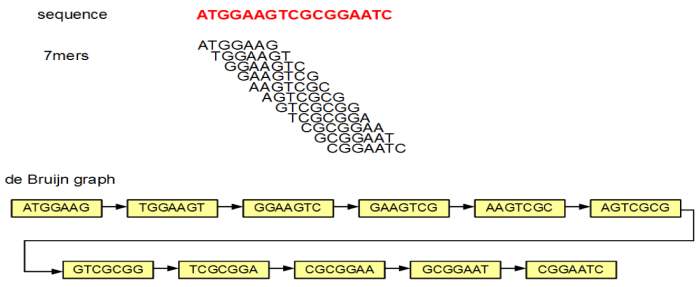
'''Figure 6:''' A simple depiction of de bruijn graph traversal. [[http://homolog.us/blogs/ Source]] | |||
The original sequence is divided into kmers, and each kmer is an node in the graph. Adjacent kmers are connected based on overlap with neighbors. But a real genome is quite unlike the example above, introductions of repeat regions complicate the problem. | |||
[[File:unicycler_repeat.png | 700px]] | |||
'''Figure 7:''' Repeat regions introduce multiple traversal paths. [[https://github.com/rrwick/Unicycler Source]] | |||
Repeats introduce ambiguity in the path the graph follows, and as the number of repeats increase, the graph becomes increasingly harder to traverse. This can be resolved by taking into account the overlap information and the multiplicity of the reads. | |||
=== | [[File:unicycler_multiplicty.png |700px]] | ||
'''Figure 8:''' Unicycler solves repeat regions by using read depth and graph connectivity to distinguish between single copy contigs and repeats. [[https://github.com/rrwick/Unicycler Source]] | |||
==== Tool testing ==== | |||
We tested 10 of the largest samples in our dataset as file size would be the speed-limiting step. We also ran each tool with default parameters as they all have methods in place that determine optimum k-mer lengths. | |||
Rationale: The following tools were chosen based on existing literature on comparisons, GAGE evaluations, and the evaluations done by the 2016 and 2017 CompGenomics assembly groups. They are debruijn graph based assemblers that differ in their algorithms based on how they handle kmers. | |||
1. '''''SPAdes''''': | |||
SPAdes uses 3 different kmer lengths to find an optimum traversal path. It also has a built in scaffolding tool that it uses to merge contigs. Detailed information on SPAdes can be found [https://www.ncbi.nlm.nih.gov/pmc/articles/PMC3342519/ here] | |||
2. '''''MaSuRCA''''': | |||
MaSuRCA combines initially constructed kmers into "super reads which tend to be longer than typical Illumina reads. The subsequent steps use these super reads instead of the initial kmers. More information can be found [https://www.biorxiv.org/content/biorxiv/early/2016/07/26/066100.full.pdf here] | |||
3. '''''Unicycler''''': | |||
Unicycler applies SPAdes assembly, but tests across a wide range of k-mer lengths. It also has several built in steps for repeat resolution, scaffolding and final polishing. This produces high qualitiy assemblies but is most time and resource consuming. More information on Unicycler can be found [http://journals.plos.org/ploscompbiol/article?id=10.1371/journal.pcbi.1005595 here] | |||
4. '''''Skesa''''': | |||
Skesa is the most recent tool in our list and is currently used by NCBI. Information about the algorithm is currently unavailable. Since Skesa does not have inbuilt scaffolding, the step for it has been added. | |||
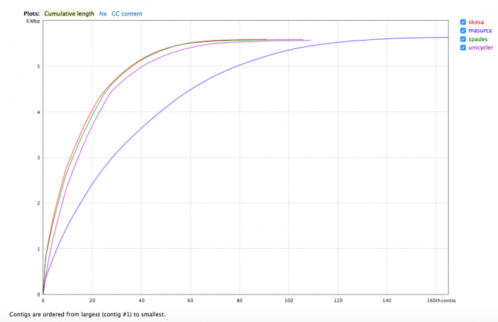
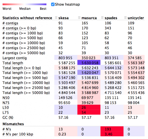
To compare the performance of the above tools, we use Quast. The results illustrated in the Figure 9. | |||
[[File: quast.png | 700px]] [[File: Quast table.png | 500px]] | |||
'''Figure 9:''' ''The above is a Quast report for one of the 10 samples in our test dataset. In terms of N50 and L50 scores, as expected Unicycler produced the best assemblies, but SPAdes and Skesa (after scaffolding) are comparable. MaSURca produced the lowest quality assemblies. '' | |||
In terms of ease of install, Skesa and SPAdes provided precompiled binaries, whereas Unicycler and MaSuRCA were uncompiled and had several prerequisites. | |||
In terms of speed, we found Skesa to be the fastest by a considerable margin. | |||
{| class="wikitable" | |||
|- | |||
! '''Tool''' | |||
! Skesa | |||
! SPAdes | |||
! MaSuRCA | |||
! Unicycler | |||
|- | |||
| Average processing time per genome (min) | |||
| ~5.5 | |||
| ~30 | |||
| ~11 | |||
| ~85 | |||
|} | |||
Based on the above results, we chose Skesa as the assembler of choice, as it produces high quality assemblies in a significantly short amount of time. | |||
== Post Assembly == | == Post Assembly == | ||
'''Improvement Scaffolding''' | |||
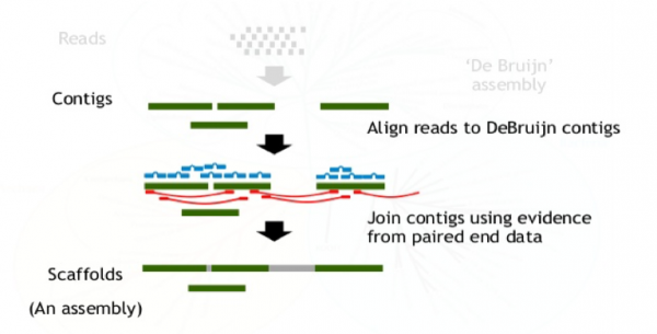
After choosing the highest quality draft assemblies, contigs would be unordered mass of stretches of DNA. To improve it, scaffolding is used to bring order and direction to these unordered DNA. The tool called SSPACE is used in this step. Using paired end data of reads, algorithm of scaffolding attempts to join multiple contigs by closing the gaps between contigs and determining the order they are in. | |||
The long reads are usually sequenced at a lower depth, whereas the short reads are sequenced at a higher depth. Both the long reads and the short reads complement each other to produce a better de novo assembly. | |||
[[File: Scafolding.png | 600px ]] | |||
'''Figure 10:''' ''Scaffolding'' | |||
'''Assessment Scoring methods''' | |||
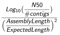
Since different assembly methods are used, post assembly steps should be done for choosing the tool that generated the best quality. N50 and L50 are some of these scoring methods. By using these scoring methods, we can determine which assembly has the highest quality. | |||
''N50 Weighted Score (Contig)'' | |||
[[File: N50.png |200px]] | |||
''L50 Weighted Score (Scaffold)'' | |||
[[File: L50.png |200px]] | |||
Simply, the better score means less number of contigs and longer length. | |||
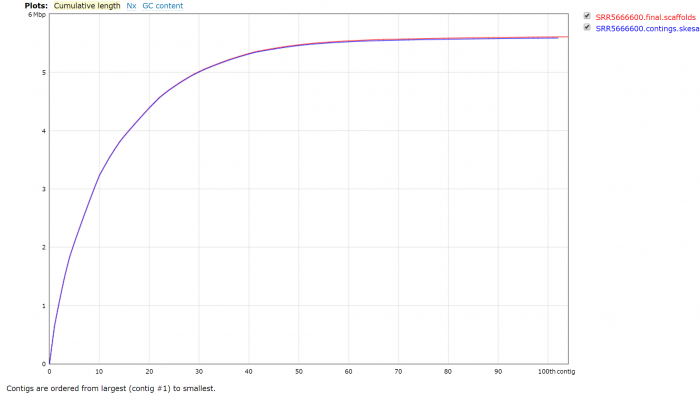
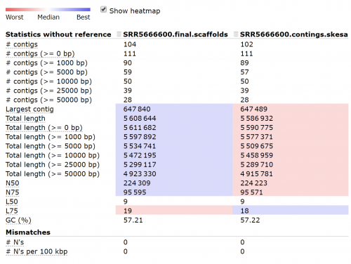
[[File: quast_sspace.png | 700px]] [[File: quast_table_sspace.png | 500px]] | |||
'''Figure 11:''' ''SSPACE shows only marginal scaffolding improvement'' | |||
== Results== | |||
=== Preliminary Genome Assembly Pipeline === | |||
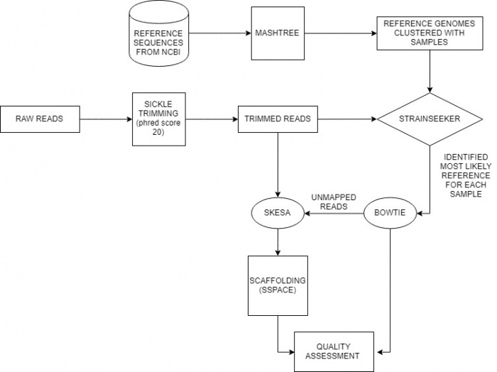
[[File: FINAL_PIPELINE1.jpg | 700px]] | |||
'''Figure 12:''' ''The pipeline that executed to carry out our final evaluations.'' | |||
===Quast comparison of de novo and reference assemblies=== | |||
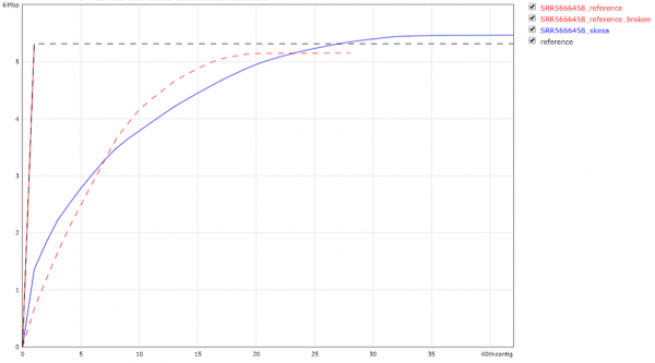
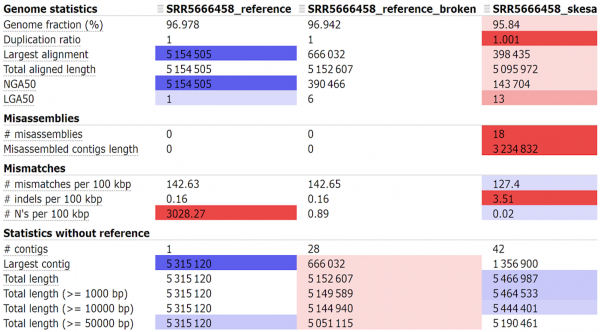
[[File:Quast comparison of de novo and reference assemblies1.png | 600px]] [[File:Quast comparison of de novo and reference assemblies2.png | 600px]] | |||
'''Figure 13:''' ''The Quast output for the sample with median genome fraction coverage'' | |||
Figure 13 shows the median sample of our de novo assembly compared with our reference assembly. The first column in the table is our bowtie2 assembled sample where reads have been merged with 'N's to preserve order when compared to a reference genome. "reference_broken" contains the un-merged reads. It is clear from the N50 scores and number of contigs that the reference alignment has produced a better quality assembly. | |||
===Distribution of genome fraction coverage=== | |||
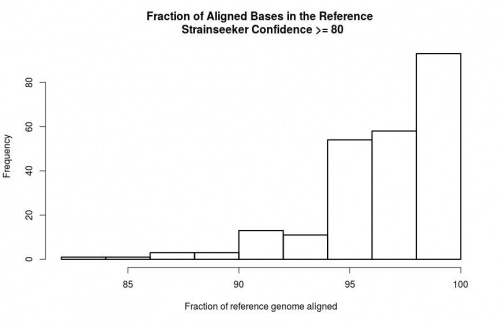
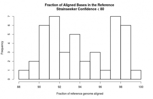
We grouped our samples based on the reference identification confidence score produced by strain seeker - Above 80% and below 80%. Figure 14 shows the distribution of genome fraction coverage for these two cases. We can see in Figure 14 (a) that most assemblies aligned with the strainseeker- recommended reference gave above 95% genome fraction coverage in the 'above 80% confidence' group. IN Figure 14 (b) The genome fraction coverage in the 'below 80% confidence' group gives a random distribution where most samples have <95% coverage. | |||
This tells us that Strainseeker's confidence scores are fairly reliable and we recommend using only >95% confidence assemblies for further processing. | |||
[[File:Distribution of genome fraction coverage1.jpg | 500px]] [[File:Distribution of genome fraction coverage2.jpg | 500px]] | |||
'''Figure 14:''' ''Distribution of genome fraction coverage '''(a)''' above 80% confidence '''(b)''' below 80% confidence'' | |||
===Assembly of unmapped reads=== | |||
As our initial database of reference sequences were built with plasmid-free genomes, it is likely that the unmapped reads from reference alignments could contain some plasmid sequences. We assembled our unmapped reads using skesa and BLASTed against NCBI's database and found that some of the unmapped reads contain plasmids. | |||
[[File:Assembly of unmapped reads.png | 700px]] | |||
==Discussion== | |||
[[File:Screenshot (101).png | 450px]] [[File:Screenshot (99).png | 450px]] | |||
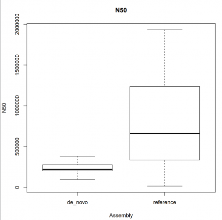
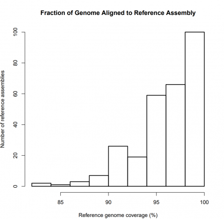
'''Figure 15:''' '''(a)''' ''Comparison of N50 in de novo and references assembly'' '''(b)''' ''Fraction of genomes aligned to reference assembly'' | |||
{| class="wikitable" | |||
|- | |||
! Alignment score | |||
! Number of samples | |||
|- | |||
| < 90% | |||
| 13 | |||
|- | |||
| >= 95% | |||
| 212 | |||
|- | |||
| >= 99% | |||
| 44 | |||
|} | |||
The distrubtion of N50 scores in reference assemblies and the number of samples that have less than 95% genome fraction coverage suggest that some samples do not have a reliable reference. We are able to provide species level information with high confidence for more than 200 out of 258 samples. However, one drawback of reference-guided assembly is that positional information such as insertions and deletions of phage and plasmids is not represented as our references are plasmid and phage-free sequences. | |||
To avoid any reference alignment associated bias and to preserve positional information with respect to phage integration sites, we have decided to submit our de novo assemblies as our final output. However we will also provide the closest reference sequence we found for each sample as we expect this information will be valuable for the annotation and comparative genomics groups. | |||
===Final Genome Assembly pipeline=== | |||
[[File:Denovopipeline.png]] | |||
== References == | |||
1. Johnson DI. Bacterial Virulence Factors. Bacterial Pathogens and Their Virulence Factors. 2017:1–38. | |||
2. Kumar V, Sun P, Vamathevan J, Li Y, Ingraham K, Palmer L, Huang J, Brown JR. Comparative Genomics of ''Klebsiella pneumoniae'' Strains with Different Antibiotic Resistance Profiles. Antimicrobial Agents and Chemotherapy. 2011;55(9):4267–4276. | |||
3. Martin M. Cutadapt removes adapter sequences from high-throughput sequencing reads. EMBnet.journal. 2011;17(1):10. | |||
4. Andrews S. (2010). FastQC: a quality control tool for high throughput sequence data. Available at http://www.bioinformatics.babraham.ac.uk/projects/fastqc. | |||
5. Joshi NA, Fass JN. (2011). Sickle: A sliding-window, adaptive, quality-based trimming tool for FastQ files (Version 1.33) [Software]. Available at https://github.com/najoshi/sickle. | |||
6. Li H, Durbin R. Fast and accurate short read alignment with Burrows-Wheeler transform. Bioinformatics. 2009;25(14):1754–1760. | |||
7. Roosaare MCA, Vaher M, Kaplinski L, Möls M, Andreson R, Lepamets M, Kõressaar T, Naaber P, Kõljalg S, Remm M. StrainSeeker: fast identification of bacterial strains from raw sequencing reads using user-provided guide trees. PeerJ. 2017;5. | |||
8. Thankachan SV, Chockalingam SP, Liu Y, Apostolico A, Aluru S. ALFRED: A Practical Method for Alignment-Free Distance Computation. Journal of Computational Biology. 2016;23(6):452–460. | |||
9. Langmead B, Salzberg SL. Fast gapped-read alignment with Bowtie 2. Nature Methods. 2012;9(4):357–359. | |||
10. Compeau PEC, Pevzner PA, Tesler G. How to apply de Bruijn graphs to genome assembly. Nature Biotechnology. 2011;29(11):987–991. | |||
11. Bankevich A, Nurk S, Antipov D, Gurevich AA, Dvorkin M, Kulikov AS, Lesin VM, Nikolenko SI, Pham S, Prjibelski AD, et al. SPAdes: A New Genome Assembly Algorithm and Its Applications to Single-Cell Sequencing. Journal of Computational Biology. 2012;19(5):455–477. | |||
12. Zimin AV, Puiu D, Luo M-C, Zhu T, Koren S, Yorke JA, Dvorak J, Salzberg S. Hybrid assembly of the large and highly repetitive genome of ''Aegilops tauschii'', a progenitor of bread wheat, with the mega-reads algorithm. 2016. | |||
13. Wick RR, Judd LM, Gorrie CL, Holt KE. Unicycler: Resolving bacterial genome assemblies from short and long sequencing reads. PLOS Computational Biology. 2017;13(6). | |||
14. Boetzer M, Henkel CV, Jansen HJ, Butler D, Pirovano W. Scaffolding pre-assembled contigs using SSPACE. Bioinformatics. 2010;27(4):578–579. | |||
15. Gurevich A, Saveliev V, Vyahhi N, Tesler G. QUAST: quality assessment tool for genome assemblies. Bioinformatics. 2013;29(8):1072–1075. | |||
Latest revision as of 18:48, 20 April 2018
Introduction
Background
Antibiotic resistance has been called one of the world’s most pressing public health problems. It is the ability of bacteria to resist the effects of an antibiotic and occurs when bacteria change in a way that reduces the effectiveness of drugs, chemicals, or other agents designed to cure or prevent infections. The bacteria survive and continue to multiply, causing more harm (Figure 1.a.). Antibiotic resistance can cause illnesses that were once easily treatable with antibiotics to become dangerous infections, prolonging suffering for children and adults. Antibiotic-resistant bacteria can spread to family members, schoolmates, and co-workers, and may threaten your community (Figure 1.b). Antibiotic-resistant bacteria are often more difficult to kill and more expensive to treat and in some cases, can lead to serious disability or even death.
Figure 1: a. How antibiotic resistance happens, b. How antibiotic resistance spreads here
Data
Emory Antibiotic Resistance Center (ARC) in Emory University, School of medicine tries to better understand antibiotic resistance to combat this crisis and improve human health. Their goals include learning how antibiotic resistance develops, optimizing the way antibiotics are used to preserve their power, and discovering novel therapeutics and vaccines to directly combat antibiotic-resistant pathogens. Solving the crisis of antibiotic resistance requires a multi-faceted approach that crosses traditional boundaries here.
Dr. David S. Weiss' lab (ARC, Division of Infectious Diseases) provided us with a sample ID numbers and we downloaded 258 pair-end raw reads sequences of Klebsiella spp,sequenced by illumina MiSeq. from NCBI SRA database.
Klebsiella is a genus of nonmotile, Gram-negative, oxidase-negative, rod-shaped bacteria (Figure 2) with a prominent polysaccharide-based capsule. Klebsiella species are found everywhere in nature. The members of the genus Klebsiella are a part of the human and animal's normal flora in the nose, mouth and intestines. The species of Klebsiella are all gram-negative and non-motile. They tend to be shorter and thicker when compared to others in the Enterobacteriaceae family. The cells are rods in shape and generally measures 0.3 to 1.5 µm wide by 0.5 to 5.0 µm long. They can be found singly, in pairs, in chains or linked end to end. Klebsiella can grow on ordinary lab medium and do not have special growth requirements, like the other members of Enterobacteriaceae. Some of Klebsiella types are: K.granulomatis, K. oxytoca, K. michiganensis and K. pneumoniae (type-species: K. p. subsp. ozaenae, K. p. subsp. pneumoniae, K. p. subsp. rhinoscleromatis) here. Though, they have been extensively studied, for example, only four complete genomes of K. pneumoniae were available till 2011 here. To better understand the multidrug resistance factors in Klebsiella, we need to determine genome DNA sequences of strains.
Figure 2: Scanning electron microscope image of Klebsiella pneumoniae. From: Bioquell.com
Objectives
The main objectives of the project is to distinguish between susceptible and heteroresistant strains/species, discover genomic determinants of antibiotic resistance and develop a predictive web server. Genome assembly group's objective, as the the first subgroup of the project, is to assemble the whole or contig genomes of DNA.
Pre-Assembly
Before doing any assembly, we would like to got some basic statistics about our dataset as:
1. Per base sequence quality
2. Per base N content
3. Per base GC content
4. Overrepresented sequences
5. Sequence length distribution
We use FastQC here for receiving these information and making some visualization. These kind of information will give us an overall view and help us to improve the quality of our sequences, if it is necessary, as raw inputs for the assemblers . For example, The presence of poor quality or technical sequences such as adapters in next-generation sequencing (NGS) data can easily affect the quality of assembly. We used Trim Galore here and Sickle here to guarantee the best performance for each assembly method that we will use.
Trim Galore is a wrapper script to automate quality and adapter trimming as well as quality control. It specifically designed for Illumina data and has an Illumina adapter library.
Sickle is a tool that uses sliding windows along with quality and length thresholds to determine when quality is sufficiently low to trim the 3'-end of reads and also determines when the quality is sufficiently high enough to trim the 5'-end of reads (Figure 3).
Figure 3: How Sickle is working
The results for before and after trimming of one of our samples shown in Figure 4.
Figure 4: Per base sequence quality and Base content of one of the sample before and after trimming
After trimming the adapter and the low quality reads, we can check the quality of all sequences at one with the MultiQC here tool.
MultiQC is a general use tool, perfect for summarising the output from numerous bioinformatics tools .
Figure 5: Summary of trimmed reads from MultiQC
Assembly
In bioinformatics, sequence assembly refers to aligning and merging fragments from a longer DNA sequence in order to reconstruct the original sequence. This is needed as DNA sequencing technology cannot read whole genomes in one go, but rather reads small pieces of between 20 and 30000 bases, depending on the technology used here.
Reference Assembly
A type of genome assembly where the reads are mapped (or compared) to a known version of the organism’s genome. It saves time and is significantly more accurate and assemble the genome with less contigs. But, it has some disadvantage too. We would not discover new genes with this method of assembly, new (completely different) sequences may lost. It requires a reference that is very similar to the sequenced data. If multiple positions on the reference genome are equally likely for a read, then, reads are ignored, placed at multiple locations or placed at the first likely position.
Tool testing
Most reference aligners use burrows-wheeler transform, which was initially developed as a compression algorithm. It is explained in detail here . We decided to compare the burrows wheeler aligner with bowtie2, which aligns short reads using a seed-and-extend method. We aligned a small subset of our samples against a reference Klebsiella pneumoniae and Klebsiella oxytoca genome.
| Bowtie2 | Klebsiella pneumoniae | Klebsiella oxytoca |
|---|---|---|
| Average time for one alignment | 17 minutes | 17 minutes |
| Genome fraction coverage | 97% | No conting larger than 7% |
| bwa | Klebsiella pneumoniae | Klebsiella oxytoca |
|---|---|---|
| Average time for one alignment | 17 minutes | 26 minutes |
| Genome fraction coverage | 97% | No conting larger than 58% |
Based on the results above, we decided to proceed with bowtie2, as we found it to be less resource intensive.
Identifying suitable reference genomes
As we don't know the species of the Klebsiella, cannot simply choose a Klebsiella species to use as reference genome. Therefore, we need to find the reference genomes from the 250+ Klebsiella genomes which are closest related to our reads. For this aim, we used Mashtree. It creates a tree based on Mash distance for our trimmed reads and 250+ Klebsiella genomes. Based on this Mashtree, we filtered to form a set of 51 representative reference. Strainseeker is the tool that we used for strain identification.
StrainSeeker is a two step process:
1) Building the database: We built a custom database with the filtered 51 references using the builder.pl script which takes input as references in fasta format and a newick reference guide tree. To generate the tree, we used ALFRED-G and converted it to a newick format for strainseeker input.
2) Strain Identification: The trimmed fastq reads (either forwards or reverse or both) are input to the seeker.pl script which looks through the reference database and infers the identity.
Results from StrainSeeker will tell us which Klebsiella strain is related to each single read. Based on these results we categorize all the reads into different bins based on the references and assemble that batch based on the assigned reference using Bowtie2.
De Novo Assembly
De novo sequencing refers to sequencing a novel genome where there is no reference sequence available for alignment. Sequence reads are assembled as contigs, and the coverage quality of de novo sequence data depends on the size and continuity of the contigs (ie, the number of gaps in the data).
We chose assemblers that follow De Bruijn graph based methods for our samples, as we are handling a large volume of samples, speed is of high priority.
De Bruijn graphs
Figure 6: A simple depiction of de bruijn graph traversal. [Source]
The original sequence is divided into kmers, and each kmer is an node in the graph. Adjacent kmers are connected based on overlap with neighbors. But a real genome is quite unlike the example above, introductions of repeat regions complicate the problem.
Figure 7: Repeat regions introduce multiple traversal paths. [Source]
Repeats introduce ambiguity in the path the graph follows, and as the number of repeats increase, the graph becomes increasingly harder to traverse. This can be resolved by taking into account the overlap information and the multiplicity of the reads.
Figure 8: Unicycler solves repeat regions by using read depth and graph connectivity to distinguish between single copy contigs and repeats. [Source]
Tool testing
We tested 10 of the largest samples in our dataset as file size would be the speed-limiting step. We also ran each tool with default parameters as they all have methods in place that determine optimum k-mer lengths.
Rationale: The following tools were chosen based on existing literature on comparisons, GAGE evaluations, and the evaluations done by the 2016 and 2017 CompGenomics assembly groups. They are debruijn graph based assemblers that differ in their algorithms based on how they handle kmers.
1. SPAdes:
SPAdes uses 3 different kmer lengths to find an optimum traversal path. It also has a built in scaffolding tool that it uses to merge contigs. Detailed information on SPAdes can be found here
2. MaSuRCA:
MaSuRCA combines initially constructed kmers into "super reads which tend to be longer than typical Illumina reads. The subsequent steps use these super reads instead of the initial kmers. More information can be found here
3. Unicycler:
Unicycler applies SPAdes assembly, but tests across a wide range of k-mer lengths. It also has several built in steps for repeat resolution, scaffolding and final polishing. This produces high qualitiy assemblies but is most time and resource consuming. More information on Unicycler can be found here
4. Skesa:
Skesa is the most recent tool in our list and is currently used by NCBI. Information about the algorithm is currently unavailable. Since Skesa does not have inbuilt scaffolding, the step for it has been added.
To compare the performance of the above tools, we use Quast. The results illustrated in the Figure 9.
Figure 9: The above is a Quast report for one of the 10 samples in our test dataset. In terms of N50 and L50 scores, as expected Unicycler produced the best assemblies, but SPAdes and Skesa (after scaffolding) are comparable. MaSURca produced the lowest quality assemblies.
In terms of ease of install, Skesa and SPAdes provided precompiled binaries, whereas Unicycler and MaSuRCA were uncompiled and had several prerequisites.
In terms of speed, we found Skesa to be the fastest by a considerable margin.
| Tool | Skesa | SPAdes | MaSuRCA | Unicycler |
|---|---|---|---|---|
| Average processing time per genome (min) | ~5.5 | ~30 | ~11 | ~85 |
Based on the above results, we chose Skesa as the assembler of choice, as it produces high quality assemblies in a significantly short amount of time.
Post Assembly
Improvement Scaffolding
After choosing the highest quality draft assemblies, contigs would be unordered mass of stretches of DNA. To improve it, scaffolding is used to bring order and direction to these unordered DNA. The tool called SSPACE is used in this step. Using paired end data of reads, algorithm of scaffolding attempts to join multiple contigs by closing the gaps between contigs and determining the order they are in.
The long reads are usually sequenced at a lower depth, whereas the short reads are sequenced at a higher depth. Both the long reads and the short reads complement each other to produce a better de novo assembly.
Figure 10: Scaffolding
Assessment Scoring methods
Since different assembly methods are used, post assembly steps should be done for choosing the tool that generated the best quality. N50 and L50 are some of these scoring methods. By using these scoring methods, we can determine which assembly has the highest quality.
N50 Weighted Score (Contig)
L50 Weighted Score (Scaffold)
Simply, the better score means less number of contigs and longer length.
Figure 11: SSPACE shows only marginal scaffolding improvement
Results
Preliminary Genome Assembly Pipeline
Figure 12: The pipeline that executed to carry out our final evaluations.
Quast comparison of de novo and reference assemblies
Figure 13: The Quast output for the sample with median genome fraction coverage
Figure 13 shows the median sample of our de novo assembly compared with our reference assembly. The first column in the table is our bowtie2 assembled sample where reads have been merged with 'N's to preserve order when compared to a reference genome. "reference_broken" contains the un-merged reads. It is clear from the N50 scores and number of contigs that the reference alignment has produced a better quality assembly.
Distribution of genome fraction coverage
We grouped our samples based on the reference identification confidence score produced by strain seeker - Above 80% and below 80%. Figure 14 shows the distribution of genome fraction coverage for these two cases. We can see in Figure 14 (a) that most assemblies aligned with the strainseeker- recommended reference gave above 95% genome fraction coverage in the 'above 80% confidence' group. IN Figure 14 (b) The genome fraction coverage in the 'below 80% confidence' group gives a random distribution where most samples have <95% coverage.
This tells us that Strainseeker's confidence scores are fairly reliable and we recommend using only >95% confidence assemblies for further processing.
Figure 14: Distribution of genome fraction coverage (a) above 80% confidence (b) below 80% confidence
Assembly of unmapped reads
As our initial database of reference sequences were built with plasmid-free genomes, it is likely that the unmapped reads from reference alignments could contain some plasmid sequences. We assembled our unmapped reads using skesa and BLASTed against NCBI's database and found that some of the unmapped reads contain plasmids.
Discussion
Figure 15: (a) Comparison of N50 in de novo and references assembly (b) Fraction of genomes aligned to reference assembly
| Alignment score | Number of samples |
|---|---|
| < 90% | 13 |
| >= 95% | 212 |
| >= 99% | 44 |
The distrubtion of N50 scores in reference assemblies and the number of samples that have less than 95% genome fraction coverage suggest that some samples do not have a reliable reference. We are able to provide species level information with high confidence for more than 200 out of 258 samples. However, one drawback of reference-guided assembly is that positional information such as insertions and deletions of phage and plasmids is not represented as our references are plasmid and phage-free sequences.
To avoid any reference alignment associated bias and to preserve positional information with respect to phage integration sites, we have decided to submit our de novo assemblies as our final output. However we will also provide the closest reference sequence we found for each sample as we expect this information will be valuable for the annotation and comparative genomics groups.
Final Genome Assembly pipeline
References
1. Johnson DI. Bacterial Virulence Factors. Bacterial Pathogens and Their Virulence Factors. 2017:1–38.
2. Kumar V, Sun P, Vamathevan J, Li Y, Ingraham K, Palmer L, Huang J, Brown JR. Comparative Genomics of Klebsiella pneumoniae Strains with Different Antibiotic Resistance Profiles. Antimicrobial Agents and Chemotherapy. 2011;55(9):4267–4276.
3. Martin M. Cutadapt removes adapter sequences from high-throughput sequencing reads. EMBnet.journal. 2011;17(1):10.
4. Andrews S. (2010). FastQC: a quality control tool for high throughput sequence data. Available at http://www.bioinformatics.babraham.ac.uk/projects/fastqc.
5. Joshi NA, Fass JN. (2011). Sickle: A sliding-window, adaptive, quality-based trimming tool for FastQ files (Version 1.33) [Software]. Available at https://github.com/najoshi/sickle.
6. Li H, Durbin R. Fast and accurate short read alignment with Burrows-Wheeler transform. Bioinformatics. 2009;25(14):1754–1760.
7. Roosaare MCA, Vaher M, Kaplinski L, Möls M, Andreson R, Lepamets M, Kõressaar T, Naaber P, Kõljalg S, Remm M. StrainSeeker: fast identification of bacterial strains from raw sequencing reads using user-provided guide trees. PeerJ. 2017;5.
8. Thankachan SV, Chockalingam SP, Liu Y, Apostolico A, Aluru S. ALFRED: A Practical Method for Alignment-Free Distance Computation. Journal of Computational Biology. 2016;23(6):452–460.
9. Langmead B, Salzberg SL. Fast gapped-read alignment with Bowtie 2. Nature Methods. 2012;9(4):357–359.
10. Compeau PEC, Pevzner PA, Tesler G. How to apply de Bruijn graphs to genome assembly. Nature Biotechnology. 2011;29(11):987–991.
11. Bankevich A, Nurk S, Antipov D, Gurevich AA, Dvorkin M, Kulikov AS, Lesin VM, Nikolenko SI, Pham S, Prjibelski AD, et al. SPAdes: A New Genome Assembly Algorithm and Its Applications to Single-Cell Sequencing. Journal of Computational Biology. 2012;19(5):455–477.
12. Zimin AV, Puiu D, Luo M-C, Zhu T, Koren S, Yorke JA, Dvorak J, Salzberg S. Hybrid assembly of the large and highly repetitive genome of Aegilops tauschii, a progenitor of bread wheat, with the mega-reads algorithm. 2016.
13. Wick RR, Judd LM, Gorrie CL, Holt KE. Unicycler: Resolving bacterial genome assemblies from short and long sequencing reads. PLOS Computational Biology. 2017;13(6).
14. Boetzer M, Henkel CV, Jansen HJ, Butler D, Pirovano W. Scaffolding pre-assembled contigs using SSPACE. Bioinformatics. 2010;27(4):578–579.
15. Gurevich A, Saveliev V, Vyahhi N, Tesler G. QUAST: quality assessment tool for genome assemblies. Bioinformatics. 2013;29(8):1072–1075.
