Team I Functional Annotation Group: Difference between revisions
| Line 173: | Line 173: | ||
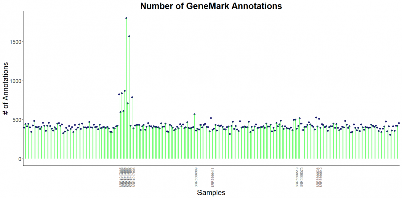
[[File:GeneMark annotations.png|800px|centre]] | [[File:GeneMark annotations.png|800px|centre]] | ||
<div style="text-align: center;">'''Figure 4. The distribution of number of GeneMark annotations for samples. The average is about 430. | <div style="text-align: center;">'''Figure 4. The distribution of number of GeneMark annotations for samples. The average is about 430. Five samples has even higher number of annotations (about 750). Two samples has even higher number of annotations (about 1000).'''</div> | ||
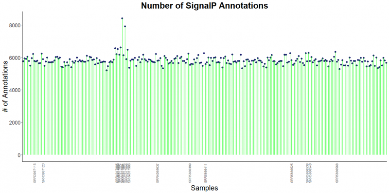
[[File:SignalP.png|800px|centre]] | [[File:SignalP.png|800px|centre]] | ||
<div style="text-align: center;">'''Figure 5. The distribution of number of SignalP annotations for samples. The average is about 5800. '''</div> | <div style="text-align: center;">'''Figure 5. The distribution of number of SignalP annotations for samples. The average is about 5800. Two samples has a higher number of annotations (about 8000).'''</div> | ||
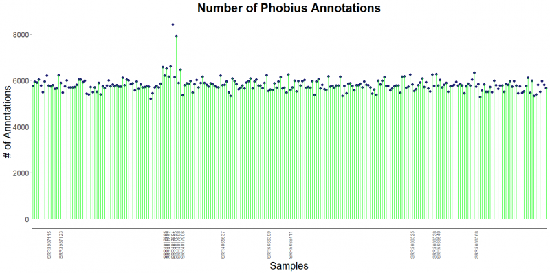
[[File:Phobius.png|800px|centre]] | [[File:Phobius.png|800px|centre]] | ||
<div style="text-align: center;">'''Figure 6. The distribution of number of Phobius annotations for samples. The average is about 5800. '''</div> | <div style="text-align: center;">'''Figure 6. The distribution of number of Phobius annotations for samples. The average is about 5800. Two samples has a higher number of annotations (about 8000).'''</div> | ||
[[File:LipoP.png|800px|centre]] | [[File:LipoP.png|800px|centre]] | ||
<div style="text-align: center;">'''Figure 7. The distribution of number of LipoP annotations for samples. The average is about 5800. '''</div> | <div style="text-align: center;">'''Figure 7. The distribution of number of LipoP annotations for samples. The average is about 5800. Two samples has a higher number of annotations (about 8000).'''</div> | ||
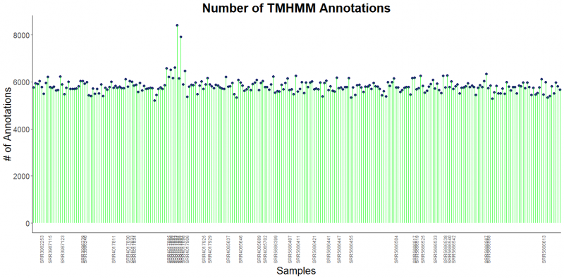
[[File:TMHMM.png|800px|centre]] | [[File:TMHMM.png|800px|centre]] | ||
<div style="text-align: center;">'''Figure 8. The distribution of number of TMHMM annotations for samples. The average is about 5800. '''</div> | <div style="text-align: center;">'''Figure 8. The distribution of number of TMHMM annotations for samples. The average is about 5800. Two samples has a higher number of annotations (about 8000).'''</div> | ||
| Line 201: | Line 201: | ||
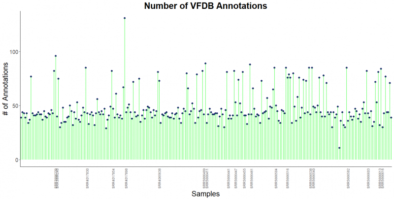
[[File:VFDB.png|800px|centre]] | [[File:VFDB.png|800px|centre]] | ||
<div style="text-align: center;">'''Figure 11. The distribution of number of VFDB annotations for samples. The average is about 50. '''</div> | <div style="text-align: center;">'''Figure 11. The distribution of number of VFDB annotations for samples. The average is about 50. One sample has a higher number of annotations (about 130).'''</div> | ||
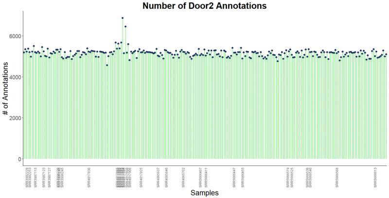
[[File:Door2.png|800px|centre]] | [[File:Door2.png|800px|centre]] | ||
<div style="text-align: center;">'''Figure 12. The distribution of number of DOOR2 annotations for samples. The average is about 5200. '''</div> | <div style="text-align: center;">'''Figure 12. The distribution of number of DOOR2 annotations for samples. The average is about 5200. Two samples has a higher number of annotations (about 6200).'''</div> | ||
====Overall Statistics==== | ====Overall Statistics==== | ||
Revision as of 22:48, 10 April 2018
Introduction
Background
Functional annotation is the process of locating genes and identifying their functions (biochemical functions, regulatory functions, etc.) in the genome. The two types of tools we used for this project are homology and ab initio. Homology based tools use databases of genetic features with known function, and accuracy is dependent on the database quality. Ab initio tools look for intrinsic characteristics of particular gene feature types and allow the tools to predict the presence of particular proteins
Objective
- Fully annotate 258 genomes from Gene Prediction group, focusing on antibiotic resistance
- Provide Comparative Genomics group with data required to perform Genome Wide Association Study(GWAS)
Pipeline
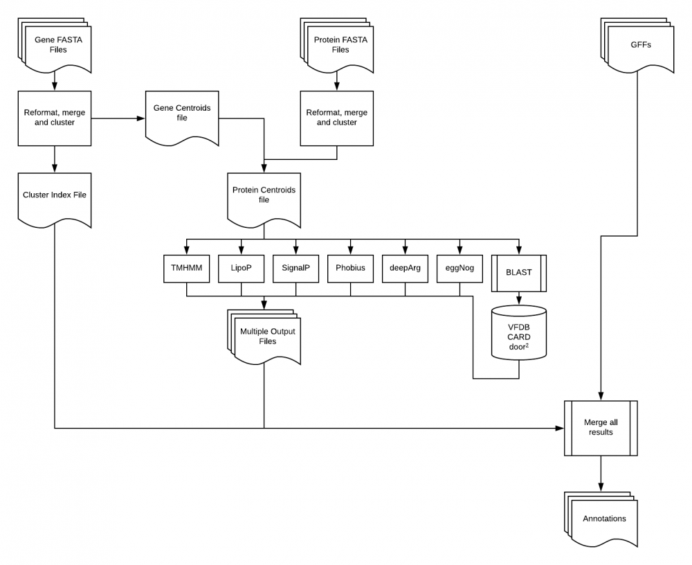
Tools
Homology
Prokka
Prokka is a command line tool that uses Prodigal(gene predictions), RNAmmer(rRNA), Aragorn(tRNA), and Infernal(non-coding RNA). Prokka is also able to add more databases to itself such as CARD and VFDB. After the genes are predicted with Prodigal they are searched through the multiple databases using blast in a hierarchical manner starting with the smallest most curated database, moving to larger domain-specific databases, and finally larger protein families databases.
Command:
prokka --outdir <output_directory> --kingdom <species' kingdom> --genus <species' genus> --gram <> --prefix <output_file> --rfam --rnammer <input_file>
- Runtime: ~ 16mins /genome
eggNOG
Eggnog performs functional annotation of genes and proteins using orthology assignments from pre-computed clusters and phylogenies from eggnog database. The database contains Orthologous Groups of proteins at taxonomic levels. Eggnog has two modes hmm and diamond that can be used. The HMM mode is comprised of a collection of precompiled hidden Markov models that have each been associated with orthologous group. Diamond is the other mode and searches for the best seed ortholog located in the eggNOG protein database. Diamond is faster than HMM thus recommended for larger datasets, but HMM is slightly more sensitive especially if the organism not well represented in the database.
Command:
python emapper.py -i <input_file> --output <output_file> -m [diamond,hmm] --usemem -d <database_name>
- --usemem: for loading the database in RAM memory
PilerCR
PilerCR identifies and analyzes CRISPR repeats
Command:
pilercr -in <input_file> -out <output_file>
- Runtime: <5 sec/genome
DeepARG
DeepARG is a machine learning solution that uses deep learning to characterize and annotate antibiotic resistance genes in metagenomes. It contains two models for different inputs, short sequence reads from Next Generation Sequencing and gene-like sequences. DeepARG outputs two files that will be mainly useful: an ARG file and a potential ARG file.
Command:
python ../deeparg-ss/deepARG.py --align --type nucl --genes --input <nucleotide.fasta> --out <output file>
python ../deeparg-ss/deepARG.py --align --type nucl --prot --input <protein.fasta> --out <output file>
- Runtime: 3min27s /genome; 44mins for our clustered nuclueotide sequences file, whose size is equivalent to ~12 genomes.
Interproscan
InterProScan runs the scanning algorithms from the InterPro database, which uses predictive models, known as signatures, provided by member databases, in an integrated way. Interproscan contains 14 databases which make up its consortium.
Databases used in final pipeline:
-PfamA: Contains many common protein domains.
-CCD: Conserved and ancient domains.
-HAMAP: Conserved protein families and subfamilies that have been manually curated.
-PROSITE: Consists of biologically significant sites, patterns, and profiles.
-SFLD: Hierarchical classification of enzymes that relate sequence-structure data to chemical capabilities.
-SMART: Identity and annotation of genetically mobile domains.
-SUPERFAMILY: Contains structural and functional annotation data for proteins and genomes.
-TIGRFAM: Protein families based on HMMs and annotation.
Command:
interproscan.sh -appl <application_you_want> -iprlookup -pa -i <input_file> -f <output_format>
- -iprlookup: include lookup of corresponding InterPro annotation in the TSV and GFF3 format
- -pa: lookup of corresponding pathway annotation
- Runtime: depends on applications you choose
DOOR2
The Database of PrOkaryotic OpeRons 2.0 (DOOR2) is the largest operon database as of April 2018. Operons are genetic units that are transcribed together and play a role in the regulation of protein synthesis based on the needs of the organism.
Workflow:
-Download operon tables from DOOR2.
-Download Fasta files based on GID
-Make a blast database and perform blastp
-Filter results and requery the operon table
(Percent identity and query coverage were filtered to be 90% or greater)
-makeblastdb -in <fasta file> -dbtype <prot or nucl>
-blastp -db <database> -query <input fasta> -out <output file> -max_target_seqs <int> -max_hsps <int> -num_threads <int> -outfmt "<int followed by information you would like presented from search>"
- Runtime: <5sec/genome, with multicore
CARD
The Comprehensive Antibiotic Resistance Database (CARD) is a database containing information of resistance genes, according resistance genes product and their associated phenotypes.
Workflow:
-Download the whole or part of the database as needed
-Make a local database using the file downloaded
-Blast the query against the database built
Command:
-makeblastdb -in <fasta file> -dbtype <prot or nucl>
-blastp -query <input fasta> -db <database> -max_hsps <int> -max_target_seqs <int> -outfmt "<int followed by information you would like presented from search>"
VFDB
The Virulence Factors Database (VFDB) is a reference database for bacterial virulence factors.
Worflow:
-Download the whole or part of the database as needed
-Make a local database using the file downloaded
-Blast the query against the database built
Command:
-makeblastdb -in <fasta file> -dbtype <prot or nucl>
-blastn -query <input fasta> -db <database> -dust <yes/no> -max_hsps <int> -max_target_seqs <int> -outfmt "<int followed by information you would like presented from search>"
Ab Initio
Phobius
Phobius predicts transmembrane topology and signal peptides from amino acid sequences, it was a challenging problem because of high similarity between the hydrophobic regions of a transmembrane helix and that of a signal peptide, leading to cross-reaction between the two types of predictions.
Phobius is based on a hidden Markov model (HMM) that models the different sequence regions of a signal peptide and the different regions of a transmembrane protein in a series of interconnected states, which allows it to have a higher accuracy rate.
Command:
phobius.pl -<output_format> <input_file> > <output_file>
- Runtime: 12-16mins /genome
LipoP
LipoP predicts lipoprotein signal peptides in Gram-negative bacteria, its hidden Markov model (HMM) was able to distinguish between lipoproteins (SPaseII-cleaved proteins), SPaseI-cleaved proteins, cytoplasmic proteins, and transmembrane proteins.
Command:
LipoP -<output_format> -<input_file> <output_file>
- Runtime: ~2mins /genome
TMHMM
TMHMM uses a hidden Markov model to predict transmembrane helices in proteins. It can discriminate between soluble and membrane proteins but has a drop in accuracy when dealing with signal peptides due to its hydrophobic region.
Command:
tmhmm -<output_format> -<input_file> <output_file>
- Runtime: ~6mins /genome
SignalP
SignalP uses a combination of several trained neural networks to predict the presence and location of signal peptide cleavage sites. SignalP allows the user to specify different types of organisms: eukaryotes or gram-positive or gram-negative prokaryotes.
Command:
signalp -t <organism_type> -f <output_format> <input_file>
- Runtime: ~ 4mins /genome
Result
Annotations
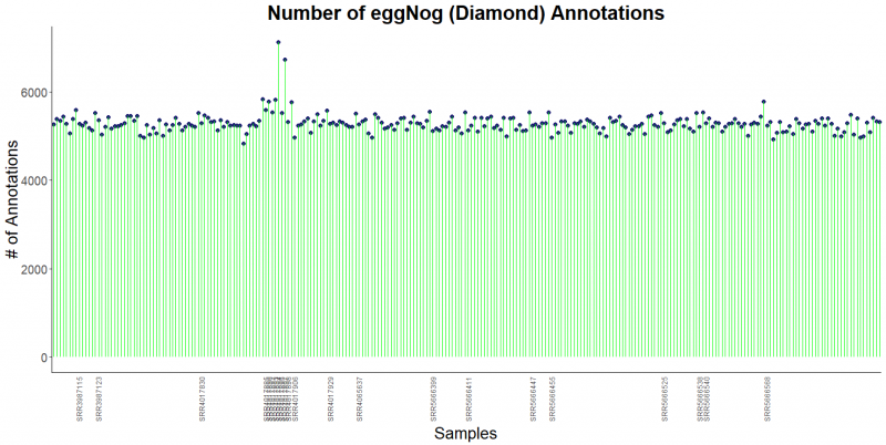
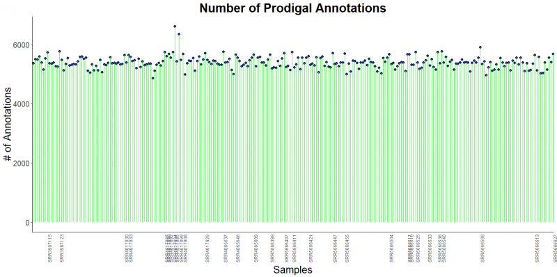

Overall Statistics
Reference
- LukasKäll, AndersKrogh, Erik L.LSonnhammer. "A Combined Transmembrane Topology and Signal Peptide Prediction Method"Journal of Molecular Biology 14 May 2004, Pages 1027-1036.
- Bendtsen, J. D., Nielsen, H., von Heijne, G., & Brunak, S. (2004). Improved prediction of signal peptides: SignalP 3.0. Journal of molecular biology, 340(4), 783-795.
- Petersen, T. N., Brunak, S., von Heijne, G., & Nielsen, H. (2011). SignalP 4.0: discriminating signal peptides from transmembrane regions. Nature methods, 8(10), 785.
- Nielsen, H. (2017). Predicting secretory proteins with SignalP. Protein Function Prediction: Methods and Protocols, 59-73.
- Jia, B., Raphenya, A. R., Alcock, B., Waglechner, N., Guo, P., Tsang, K. K., … McArthur, A. G. (2017). CARD 2017: expansion and model-centric curation of the comprehensive antibiotic resistance database. Nucleic Acids Research, 45(Database issue), D566–D573. http://doi.org/10.1093/nar/gkw1004
- Jones, P., Binns, D., Chang, H.-Y., Fraser, M., Li, W., McAnulla, C., … Hunter, S. (2014). InterProScan 5: genome-scale protein function classification. Bioinformatics, 30(9), 1236–1240. http://doi.org/10.1093/bioinformatics/btu031
- Arango-Argoty, G., Garner, E., Pruden, A., Heath, L. S., Vikesland, P., & Zhang, L. (2018). DeepARG: a deep learning approach for predicting antibiotic resistance genes from metagenomic data. Microbiome, 6(1), 23.
- Conesa, A., & Götz, S. (2008). Blast2GO: A comprehensive suite for functional analysis in plant genomics. International journal of plant genomics, 2008.
- Juncker, A. S., Willenbrock, H., Von Heijne, G., Brunak, S., Nielsen, H., & Krogh, A. (2003). Prediction of lipoprotein signal peptides in Gram‐negative bacteria. Protein Science, 12(8), 1652-1662.
- The UniProt Consortium. (2015). UniProt: a hub for protein information. Nucleic Acids Research, 43(Database issue), D204–D212. http://doi.org/10.1093/nar/gku989
- J Mol Biol. 2001 Jan 19;305(3):567-80. Predicting transmembrane protein topology with a hidden Markov model: application to complete genomes. Krogh A1, Larsson B, von Heijne G, Sonnhammer EL.
- Nguyen, M., Brettin, T., Long, S. W., Musser, J. M., Olsen, R. J., Olson, R., … Davis, J. J. (2018). Developing an in silico minimum inhibitory concentration panel test for Klebsiella pneumoniae. Scientific Reports, 8, 421. http://doi.org/10.1038/s41598-017-18972-w
- Torsten Seemann; Prokka: rapid prokaryotic genome annotation, Bioinformatics, Volume 30, Issue 14, 15 July 2014, Pages 2068–2069, https://doi.org/10.1093/bioinformatics/btu153