Team I Gene Prediction Group

Team members: Genevieve Brandt, Victoria Caban, Yuntian He, Junyu Li, Yiqiuyi Liu, Yihao Ou, Wenyi Qiu, Casey Smith, Mohit Thakur, Stephen Wist, Qinyu Yue

Introduction

Data

We were given assemblies of 258 isolates of Klebsiella spp..

Background

Our overarching goal is to understand what causes heteroresistance in Klebsiella spp. At this step, our objective was, given assembled genomes, to predict genes for Klebsiella that could later be annotated to understand functionality.

Gene Prediction

Gene prediction is the process of identifying the specific regions of genomic DNA that encode for genes. After sequencing and assembly, gene prediction is one of the first steps in understanding the genome of a species. In the past, confirming that the gene prediction is accurate demanded in vivo experimentation through gene knockout and other assays. Today, bioinformatics research has made it possible to predict the function of a gene based on its sequence alone. There are two general methods to do this: homology-based tools and ab-initio tools.

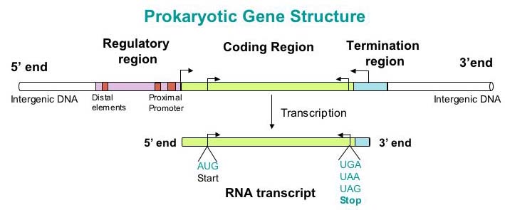
There is a big difference between prokaryotic and eukaryotic gene prediction. For eukaryotes, genes may be separated by introns, which makes it challenging to find the whole genomic sequence. Promoter sequences are more complex and less well understood in eukaryotes as well. In prokaryotes, the promoter regions are well understood, which is useful when using ab initio tools, since these tools search for signs of specific signs of protein coding genes. In prokaryotic genomes there are also contiguous open reading frames (ORFs) - when paired with the high amount of stop codons in prokaryotes this can indicate, with high probability, a gene being present. Our challenge when looking at ORFs is that every gene is a ORF, but not every ORF is a gene.

Methods

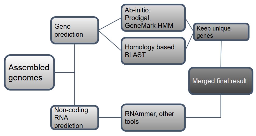
Pipeline (general workflow)

Ab-initio Methods

Ab-initio tools always predict genes based on the gene content and signal detection(e.g. start/stop codon; Ribosome Biding Site, RBS etc.). In another words, they predict genes by analyzing statistical features of genes first, then separate the coding sequences and non-coding sequences apart.

There are so many different algorithms among different ab-initio tools. For example, Dynamic programming gene finding, Hidden Markov Model, Interpolated Markov Model, Linear Discriminant Analysis and so on. By comparing the sensitive, PPV and running time, we chose some tools below to generate our final results.

Prodigal

Pros:

Straightforward installation and use

Accuracy: sensitivity - 94.7%, positive predictive value - 94.1%. Comparable to other tools

Speed: averaged 17 seconds/genome

Cons:

Fairly limited number of options

Parameters used:

mode: normal mode (DEFAULT-single genome, any number of sequences)

translation table: 4 (DEFAULT-standard bacteria, archaea) and 11 (DEFAULT-mycoplasma/spiroplasma)

gap mode: 0 (DEFAULT-partial genes run into gaps)

output format: gff (GFF format for the gene coordinates file)

rbs motif: (DEFAULT-looks for default Shine-Dalgarno motif)

Input: assembly file (.fna) Output: gene coordinates (.gff), nucleotide sequences (.fna), protein sequences (.fna) Command:

prodigal -i input.fna -o output.gff -f gff -d nucleotide_seq.fna -a protein_seq.fna

Reference: Hyatt, Doug, et al. "Prodigal: prokaryotic gene recognition and translation initiation site identification." BMC bioinformatics 11.1 (2010): 119.

Genemark.hmm

Before running GeneMark.hmm, it is necessary to got a mode file first. One way is to download the models from GeneMark website(http://opal.biology.gatech.edu/GeneMark/). Or you can generated them by GeneMarkS or GeneMark.

Pros:

easy to install and use

Accuracy: sensitivity - 93.11%, positive predictive value - 93.10%. Comparable to other tools

Speed: averaged 1.71 seconds/genome

Parameters used:

motif:1

Input: assembly file (.fna) Output: gene coordinates (.gff), nucleotide sequences (.fna), protein sequences (.fna) Command:

gmhmmp -o <output.gff> -f G -m <model with its path> <input_file> 

Reference: http://opal.biology.gatech.edu/GeneMark/background.html

Lukashin, Alexander V., and Mark Borodovsky. "GeneMark. hmm: new solutions for gene finding." Nucleic acids research 26.4 (1998): 1107-1115.

GLLIMMER

Run_glimmer.sh includes:

1. Add GLIMMER executables to PATH
2. Create output and log directories GFF/ and logs/
3. GLIMMER calling, done through a pipeline script GLIMMER3 provides g3-from-scratch.csh
4. Convert GLIMMER outputs to GFFs

Parameters used: (default in g3-from-scratch.csh)

-o 50: max prediction overlap length

-g 110: min gene length

-t 30: max entropy distance score

-d 7 : depth of interpolated context model

-p 3: period of interpolated context model

-w 12: width of interpolated context model

Input: directory of assembly FASTA file(s) Output: Gene table (.predict and .detail) and byproducts (.icm, .train, .longorfs) Command:

 bash run_glimmer.sh [directory] 

Reference: https://ccb.jhu.edu/software/glimmer/glim302notes.pdf

ncRNA Methods

Infernal

Command:

cmscan --tblout <path to write tblout file> <cm file> <input fasta> > <path to write cmscan output>

Aragorn

Command:

./aragorn -t <input file> 

References

https://ghr.nlm.nih.gov/primer/basics/gene

https://www.biostat.wisc.edu/bmi776/spring-15/lectures/IMMs.pdf

http://ece.drexel.edu/gailr/ECE-S690-503/markov_models.ppt.pdf

http://onlinelibrary.wiley.com/doi/10.1042/BC20070137/full#footer-citing

https://iweb.langara.bc.ca/biology/mario/Biol2315notes/biol2315chap11.h